rpmak
Put together rational spline
Syntax
rp = rpmak(breaks,coefs)

rp = rpmak(breaks,coefs,d)

rpmak(breaks,coefs,sizec)

rs = rsmak(knots,coefs)

rs
= rsmak(shape,parameters)
Description
Both rpmak and rsmak put together a rational spline from minimal information. rsmak is also equipped to provide rational splines that describe standard geometric shapes. A rational spline must be scalar- or vector-valued.
rp = rpmak(breaks,coefs) has the same effect as the command ppmak(breaks, coefs) except that the resulting ppform is tagged as a rational spline, i.e., as a rpform.
To describe what this means, let R be the piecewise-polynomial put together by the command ppmak(breaks,coefs), and let r(x) = s(x)/w(x) be the rational spline put together by the command rpmak(breaks,coefs). If v is the value of R at x, then v(1:end-1)/v(end) is the value of r at x. In other words, R(x) = [s(x);w(x)]. Correspondingly, the dimension of the target of r is one less than the dimension of the target of R. In particular, the dimension (of the target) of R must be at least 2, i.e., the coefficients specified by coefs must be d-vectors with d > 1. See ppmak for how the input arrays breaks and coefs are being interpreted, hence how they are to be specified in order to produce a particular piecewise-polynomial.
rp = rpmak(breaks,coefs,d) has the same effect as ppmak(breaks,coefs,d+1), except that the resulting ppform is tagged as being a rpform. Note that the desire to have that optional third argument specify the dimension of the target requires different values for it in rpmak and ppmak for the same coefficient array coefs.
rpmak(breaks,coefs,sizec) has the same effect as ppmak(breaks,coefs,sizec) except that the resulting ppform is tagged as being a rpform, and the target dimension is taken to be sizec(1)-1.
rs = rsmak(knots,coefs) is similarly related to spmak(knots,coefs), and rsmak(knots,coefs,sizec) to spmak(knots,coefs,sizec). In particular, rsmak(knots,coefs) puts together a rational spline in B-form, i.e., it provides a rBform. See spmak for how the input arrays knots and coefs are being interpreted, hence how they are to be specified in order to produce a particular piecewise-polynomial.
rs
= rsmak(shape,parameters)
provides a rational spline in rBform that describes the shape being specified by the character vector or string scalar shape and the optional additional parameters. Specific choices are:
rsmak('arc',radius,center,[alpha,beta])
rsmak('circle',radius,center)
rsmak('cone',radius,halfheight)
rsmak('cylinder',radius,height)
rsmak('southcap',radius,center)
rsmak('torus',radius,ratio)
with 1 the default value for radius, halfheight and height, and the origin the default for center, and the arc running through all the angles from alpha to beta (default is [-pi/2,pi/2]), and the cone, cylinder, and torus centered at the origin with their major circle in the (x,y)-plane, and the minor circle of the torus having radius radius*ratio, the default for ratio being 1/3.
From these, one may generate related shapes by affine transformations, with the help of fncmb(rs,transformation).
All fn... commands except fnint, fnder, fndir can handle rational splines.
Examples
The commands
runges = rsmak([-5 -5 -5 5 5 5],[1 1 1; 26 -24 26]);
rungep = rpmak([-5 5],[0 0 1; 1 -10 26],1);
both provide a description of the rational polynomial r(x) = 1/(x2 + 1) on the interval [-5 .. 5]. However, outside the interval [-5 .. 5], the function given by runges is zero, while the rational spline given by rungep agrees with 1/(x2 + 1) for every x.
The figure of a rotated cone is generated by the commands
fnplt(fncmb(rsmak('cone',1,2),[0 0 -1;0 1 0;1 0 0]))
axis equal, axis off, shading interp
A Rotated Cone Given by a Rational Quadratic Spline

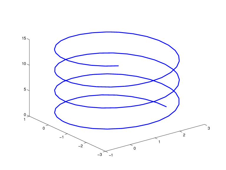
A Helix, showing a helix with several windings, is generated by the commands
arc = rsmak('arc',2,[1;-1],[0 7.3*pi]);
[knots,c] = fnbrk(arc,'k','c');
helix = rsmak(knots, [c(1:2,:);aveknt(knots,3).*c(3,:);
c(3,:)]);
fnplt(helix)
A Helix

For further illustrated examples, see NURBS and Other Rational Splines