alphaCROWNOptions

Options for α-CROWN verification

Since R2026a

Description

Add-On Required: This feature requires the AI Verification Library for Deep Learning Toolbox add-on.

Use an AlphaCROWNOptions object to set options for the α-CROWN verifier. You can use the AlphaCROWNOptions object as input to the estimateNetworkOutputBounds and verifyNetworkRobustness functions.

α-CROWN is an algorithm for neural network verification. The algorithm uses an Adam solver to optimize the bound propagation through the neural network and produce bounds on the output of a neural network. α-CROWN bounds are typically tighter than CROWN bounds. You can use these bounds to assess the robustness of your neural network to input perturbations. For more information, see CROWN and α-CROWN.

Creation

Syntax

options = alphaCROWNOptions

options = alphaCROWNOptions(Property=Value)

Description

options = alphaCROWNOptions returns optimization options for the α-CROWN algorithm. To use α-CROWN to estimate the output bounds of a regression neural network, use the options object as input to the estimateNetworkOutputBounds function. To use α-CROWN to verify the robustness of a classification neural network, use the options object as input to the verifyNetworkRobustness function.

example

options = alphaCROWNOptions(Property=Value) returns α-CROWN options with additional options specified by one or more name-value arguments.

example

Properties

expand all

Adam Solver Options

`InitialLearnRate` — Initial learning rate
`0.95` (default) | positive scalar

Initial learning rate used for parameter optimization, specified as a positive scalar.

If the learning rate is too low, then the optimization can take a long time. If the learning rate is too high, then the algorithm might reach a suboptimal result or diverge.

`MaxEpochs` — Maximum number of epochs
`10` (default) | positive integer

Maximum number of epochs (full passes of the data) to use for parameter optimization, specified as a positive integer.

`LearnRateSchedule` — Learning rate schedule
`"none"` (default) | character vector | string array | built-in or custom learning rate schedule object | function handle | cell array

Learning rate schedule, specified as a character vector or string scalar of a built-in learning rate schedule name, a string array of names, a built-in or custom learning rate schedule object, a function handle, or a cell array of names, metric objects, and function handles.

Built-In Learning Rate Schedule Names

Specify learning rate schedules as a string scalar, character vector, or a string or cell array of one or more of these names:

Name	Description	Plot
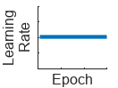
`"none"`	No learning rate schedule. This schedule keeps the learning rate constant.
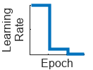
`"piecewise"`	Piecewise learning rate schedule. Every 10 epochs, this schedule drops the learn rate by a factor of 10.
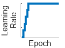
`"warmup"`	Warm-up learning rate schedule. For 5 iterations, this schedule ramps up the learning rate to the base learning rate.
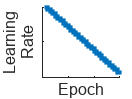
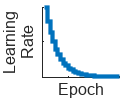
`"polynomial"`	Polynomial learning rate schedule. Every epoch, this schedule drops the learning rate using a power law with a unitary exponent.
`"exponential"`	Exponential learning rate schedule. Every epoch, this schedule decays the learning rate by a factor of `10`.
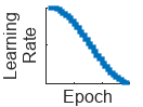
`"cosine"`	Cosine learning rate schedule. Every epoch, this schedule drops the learn rate using a cosine formula.
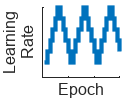
`"cyclical"`	Cyclical learning rate schedule. For periods of 10 epochs, this schedule increases the learning rate from the base learning rate for 5 epochs and then decreases the learning rate for 5 epochs.

Built-In Learning Rate Schedule Object

If you need more flexibility than what the string options provide, you can use built-in learning rate schedule objects:

piecewiseLearnRate — A piecewise learning rate schedule object drops the learning rate periodically by multiplying it by a specified factor. Use this object to customize the drop factor and period of the piecewise schedule.
warmupLearnRate — A warm-up learning rate schedule object ramps up the learning for a specified number of iterations. Use this object to customize the initial and final learning rate factors and the number of steps of the warm up schedule.
polynomialLearnRate — A polynomial learning rate schedule drops the learning rate using a power law. Use this object to customize the initial and final learning rate factors, the exponent, and the number of steps of the polynomial schedule.
exponentialLearnRate — An exponential learning rate schedule decays the learning rate by a specified factor. Use this object to customize the drop factor and period of the exponential schedule.
cosineLearnRate — A cosine learning rate schedule object drops the learning rate using a cosine curve and incorporates warm restarts. Use this object to customize the initial and final learning rate factors, the period, and the period growth factor of the cosine schedule.
cyclicalLearnRate — A cyclical learning rate schedule periodically increases and decreases the learning rate. Use this option to customize the maximum factor, period, and step ratio of the cyclical schedule.

Custom Learning Rate Schedule

For additional flexibility, you can define a custom learning rate schedule as a function handle or custom class that inherits from deep.LearnRateSchedule.

Custom learning rate schedule function handle — If the learning rate schedule you need is not a built-in learning rate schedule, then you can specify custom learning rate schedules using a function handle. To specify a custom schedule, use a function handle with the syntax learningRate = f(baseLearningRate,epoch), where baseLearningRate is the base learning rate, and epoch is the epoch number.
Custom learn rate schedule object — If you need more flexibility that what function handles provide, then you can define a custom learning rate schedule class that inherits from deep.LearnRateSchedule.

Multiple Learning Rate Schedules

You can combine multiple learning rate schedules by specifying multiple schedules as a string or cell array and then the software applies the schedules in order, starting with the first element. At most one of the schedules can be infinite (schedules than continue indefinitely, such as "cyclical" and objects with the NumSteps property set to Inf) and the infinite schedule must be the last element of the array.

`LearnRateDropPeriod` — Number of epochs for dropping the learning rate
`10` (default) | positive integer

Number of epochs for dropping the learning rate, specified as a positive integer. This argument is valid only when the LearnRateSchedule value is "piecewise".

The software multiplies the global learning rate with the drop factor every time the specified number of epochs passes. Specify the drop factor using the LearnRateDropFactor argument.

`LearnRateDropFactor` — Factor for dropping the learning rate
`0.1` (default) | scalar from `0` to `1`

Factor for dropping the learning rate, specified as a scalar from 0 to 1. This argument is valid only when the LearnRateSchedule argument is "piecewise".

LearnRateDropFactor is a multiplicative factor to apply to the learning rate every time a certain number of epochs passes. Specify the number of epochs using the LearnRateDropPeriod argument.

`GradientDecayFactor` — Decay rate of gradient moving average
`0.9` (default) | nonnegative scalar less than `1`

Decay rate of gradient moving average for the Adam solver, specified as a nonnegative scalar less than 1. The gradient decay rate is denoted by λ₁ in the Adaptive Moment Estimation section.

The default value works well for most tasks.

`SquaredGradientDecayFactor` — Decay rate of squared gradient moving average
`0.999` (default) | nonnegative scalar less than `1`

Decay rate of squared gradient moving average for the Adam solver, specified as a nonnegative scalar less than 1. The squared gradient decay rate is denoted by λ₂ in the Adaptive Moment Estimation section.

Typical values of the decay rate are 0.9, 0.99, and 0.999, corresponding to averaging lengths of 10, 100, and 1000 parameter updates, respectively.

`Epsilon` — Denominator offset
`1e-8` (default) | positive scalar

Denominator offset for Adam solver, specified as a positive scalar.

The solver adds the offset to the denominator in the neural network parameter updates to avoid division by zero. The default value works well for most tasks.

`MiniBatchSize` — Size of mini-batch
128 (default) | positive integer

Size of the mini-batch to use when verifying robustness, specified as a positive integer.

Larger mini-batch sizes require more memory, but can lead to faster computations.

`GradientThreshold` — Gradient threshold
`Inf` (default) | positive scalar

Gradient threshold, specified as Inf or a positive scalar. If the gradient exceeds the value of GradientThreshold, then the gradient is clipped according to the GradientThresholdMethod argument.

For more information, see Gradient Clipping.

`GradientThresholdMethod` — Gradient threshold method
`"l2norm"` (default) | `"global-l2norm"` | `"absolute-value"`

Gradient threshold method used to clip gradient values that exceed the gradient threshold, specified as one of the following:

"l2norm" — If the L₂ norm of the gradient of a learnable parameter is larger than GradientThreshold, then scale the gradient so that the L₂ norm equals GradientThreshold.
"global-l2norm" — If the global L₂ norm, L, is larger than GradientThreshold, then scale all gradients by a factor of GradientThreshold/L. The global L₂ norm considers all learnable parameters.
"absolute-value" — If the absolute value of an individual partial derivative in the gradient of a learnable parameter is larger than GradientThreshold, then scale the partial derivative to have magnitude equal to GradientThreshold and retain the sign of the partial derivative.

For more information, see Gradient Clipping.

Monitoring

`Verbose` — Flag to display optimization progress
`1` (`true`) (default) | `0` (`false`)

Flag to display optimization progress, specified as a numeric or logical 1 (true) or 0 (false). When you set this input to 1 (true), the function returns the progress of the algorithm by indicating which mini-batch the function is processing and the total number of mini-batches. The function also returns the options that the algorithm uses and the amount of time computation takes.

Hardware

`ExecutionEnvironment` — Hardware resource
`"auto"` (default) | `"cpu"` | `"gpu"` | `"multi-gpu"` | `"parallel-auto"` | `"parallel-cpu"` | `"parallel-gpu"`

Hardware resource for verifying network robustness, specified as one of these values:

"auto" – Use a local GPU if one is available. Otherwise, use the local CPU.
"cpu" – Use the local CPU.
"gpu" – Use the local GPU.
"multi-gpu" – Use multiple GPUs on one machine, using a local parallel pool based on your default cluster profile. If there is no current parallel pool, the software starts a parallel pool with pool size equal to the number of available GPUs.
"parallel-auto" – Use a local or remote parallel pool. If there is no current parallel pool, the software starts one using the default cluster profile. If the pool has access to GPUs, then only workers with a unique GPU perform the computations and excess workers become idle. If the pool does not have GPUs, then the computations take place on all available CPU workers instead.
"parallel-cpu" – Use CPU resources in a local or remote parallel pool, ignoring any GPUs. If there is no current parallel pool, the software starts one using the default cluster profile.
"parallel-gpu" – Use GPUs in a local or remote parallel pool. Excess workers become idle. If there is no current parallel pool, the software starts one using the default cluster profile.

The "gpu", "multi-gpu", "parallel-auto", "parallel-cpu", and "parallel-gpu" options require Parallel Computing Toolbox™. To use a GPU for deep learning, you must also have a supported GPU device. For information on supported devices, see GPU Computing Requirements (Parallel Computing Toolbox). If you choose one of these options and Parallel Computing Toolbox or a suitable GPU is not available, then the software returns an error.

For more information on when to use the different execution environments, see Scale Up Deep Learning in Parallel, on GPUs, and in the Cloud.

Objective Options

`Objective` — Objective to optimize
`"auto"` (default) | `"lower"` | `"upper"` | `"interval"`

Objective to optimize, specified as one of these values:

"auto" — Optimize the upper-lower bound interval ("interval") when using the object with the estimateNetworkOutputBounds function. Optimize only the lower bounds ("lower") when using the object with the verifyNetworkRobustness function.
"lower" — Optimize only the lower bounds.
"upper" — Optimize only the upper bounds.
"interval" — Optimize the upper-lower bound interval.

Tip

The verifyNetworkRobustness function checks for classification robustness by computing the difference in class probabilities between the true and target label probabilities. To check for robustness, it is enough to check that the lower bound of this difference is greater than 0.

Data Types: char | string

`ObjectiveMode` — Objective output mode
`"auto"` (default) | `"individual"` | `"average"`

Objective output mode, specified as:

"auto" — Optimize each objective ("individual") when using the object with the estimateNetworkOutputBounds or verifyNetworkRobutsness functions.
"average" — Optimize the average objective specified by Objective, for example, maximize the average lower bound. This reduces memory and run time use but can result in looser bounds.
"individual" — Optimize each objective specified by Objective, for example, maximize each lower bound. This increases memory use and run time but can result in tighter bounds.

Data Types: char | string

`ObjectiveModeEnvironment` — Objective mode environment
`"auto"` (default) | `"sequential"` | `"batched"`

This option is only valid when ObjectiveMode is set to "individual".

Objective mode environment, specified as:

"auto" — Optimize in a single batch ("batched") when using the object with the estimateNetworkOutputBounds and verifyNetworkRobutsness functions.
"sequential" — Optimize each objective specified by Objective sequentially, for example, maximize each lower bound one at a time. This option reduces memory use but increases run time.
"batched" — Optimize each objective specified by Objective in a single batch computation, for example, maximize each lower bound all at once. This option reduces run time but increases memory usage.

The objective mode environment value does not change the returned results.

Data Types: char | string

Object Functions

`verifyNetworkRobustness`	Verify adversarial robustness of MATLAB, ONNX, and PyTorch networks
`estimateNetworkOutputBounds`	Compute output bounds of MATLAB, ONNX, and PyTorch networks

Examples

collapse all

Specify α-CROWN Options

This example uses:

Open Live Script

Create an AlphaCROWNOptions object.

options = alphaCROWNOptions( ...
    InitialLearnRate=0.001, ...
    MaxEpochs=20, ...
    ObjectiveMode="average", ...
    Objective="upper", ...
    MiniBatchSize=16)

options = 
  AlphaCROWNOptions with properties:

                 MiniBatchSize: 16
          ExecutionEnvironment: 'auto'
              InitialLearnRate: 1.0000e-03
                     MaxEpochs: 20
                     Objective: "upper"
                 ObjectiveMode: "average"
        ObjectiveExecutionMode: 'auto'
             LearnRateSchedule: 'none'
           LearnRateDropFactor: 0.1000
           LearnRateDropPeriod: 10
           GradientDecayFactor: 0.9000
              L2Regularization: 1.0000e-04
       GradientThresholdMethod: 'l2norm'
             GradientThreshold: Inf
    SquaredGradientDecayFactor: 0.9990
                       Epsilon: 1.0000e-08
                       Verbose: 0

Verify Network Robustness Using Alpha-CROWN

This example uses:

Open Live Script

Load a pretrained classification network.

load("digitsRobustClassificationConvolutionNet.mat")

Load the test data.

[XTest,TTest] = digitTest4DArrayData;

Randomly select images to test.

idx = randi(numel(TTest),500,1);

X = XTest(:,:,:,idx);
labels = TTest(idx);

Convert the test data to a dlarray object.

X = dlarray(X,"SSCB");

Verify the network robustness to an input perturbation between –0.01 and 0.01 for each pixel. Create lower and upper bounds for the input.

perturbation = 0.01;
XLower = X - perturbation;
XUpper = X + perturbation;

Create an AlphaCROWN options object. Optimize the interval and optimize over the average objective.

opts = alphaCROWNOptions(InitialLearnRate=0.9,MaxEpochs=20, ...
    Objective="interval", ...
    ObjectiveMode="average", ...
    Verbose=true);

Verify the network robustness for each test image.

result = verifyNetworkRobustness(netRobust,XLower,XUpper,labels,Algorithm=opts);

Number of mini-batches to process: 4
.... (4 mini-batches)
Total time = 242.6 seconds.

summary(result,Statistics="counts")

result: 500×1 categorical

     verified      493 
     violated        2 
     unproven        5

Estimate Output Bounds Using Custom Optimizer

This example uses:

Open Live Script

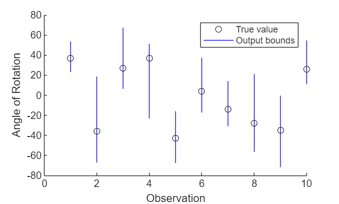
Load a pretrained regression network. This network is a dlnetwork object that has been trained to predict the rotation angle of images of handwritten digits.

load("digitsRegressionNetwork.mat");

Load the test data.

[XTest,~,TTest] = digitTest4DArrayData;

Select the first ten images.

X = XTest(:,:,:,1:10);
T = TTest(1:10);

Convert the test images to dlarray objects.

X = dlarray(X,"SSCB");

Estimate the output bounds for an input perturbation between –0.01 and 0.01 for each pixel. Create lower and upper bounds for the input.

perturbation = 0.01;
XLower = X - perturbation;
XUpper = X + perturbation;

Create an AlphaCROWN options object. Optimize the upper bound and optimize over the average objective.

opts = alphaCROWNOptions(InitialLearnRate=0.9,MaxEpochs=20, ...
    Objective="upper", ...
    ObjectiveMode="average", ...
    Verbose=true);

Estimate the output bounds for each input.

[YLower,YUpper] = estimateNetworkOutputBounds(net,XLower,XUpper);

The output bounds are dlarray objects. To plot the output bounds, first extract the data using extractdata.

YLower = extractdata(YLower);
YUpper = extractdata(YUpper);

Visualize the output bounds.

figure
hold on
for i = 1:10
    plot(i,T(i),"ko")
    line([i i],[YLower(i) YUpper(i)],Color="b")
end
hold off
xlim([0 10])
xlabel("Observation")
ylabel("Angle of Rotation")
legend(["True value","Output bounds"])

Algorithms

expand all

Adaptive Moment Estimation

Adaptive moment estimation (Adam) [1] uses a parameter update that is similar to RMSProp, but with an added momentum term. It keeps an element-wise moving average of both the parameter gradients and their squared values,

$m_{ℓ} = λ_{1} m_{ℓ - 1} + (1 - λ_{1}) \nabla E (θ_{ℓ})$

$v_{ℓ} = λ_{2} v_{ℓ - 1} + (1 - λ_{2}) {[\nabla E (θ_{ℓ})]}^{2}$

The λ₁ and λ₂ decay rates are the gradient decay and squared gradient decay factors, respectively. Adam uses the moving averages to update the network parameters as

$θ_{ℓ + 1} = θ_{ℓ} - \frac{γ m_{l}}{\sqrt{v_{l}} + ϵ}$

The value γ is the learning rate. If gradients over many iterations are similar, then using a moving average of the gradient enables the parameter updates to pick up momentum in a certain direction. If the gradients contain mostly noise, then the moving average of the gradient becomes smaller, and so the parameter updates become smaller too. The full Adam update also includes a mechanism to correct a bias that appears in the beginning of training. For more information, see [1].

Gradient Clipping

If the gradients increase in magnitude exponentially, then the optimization is unstable and can diverge within a few iterations. This "gradient explosion" is indicated by a loss that goes to NaN or Inf. Gradient clipping helps prevent gradient explosion by stabilizing the optimization at higher learning rates and in the presence of outliers [2].

There are two types of gradient clipping.

Norm-based gradient clipping rescales the gradient based on a threshold, and does not change the direction of the gradient. The "l2norm" and "global-l2norm" values of GradientThresholdMethod are norm-based gradient clipping methods.
Value-based gradient clipping clips any partial derivative greater than the threshold, which can result in the gradient arbitrarily changing direction. Value-based gradient clipping can have unpredictable behavior, but sufficiently small changes do not cause the algorithm to diverge. The "absolute-value" value of GradientThresholdMethod is a value-based gradient clipping method.

CROWN and α-CROWN

CROWN (equivalently DeepPoly) and alpha-CROWN are algorithms for neural network verification that use abstract interpretation to prove properties of the neural networks [3], [4], [5], [6].

References

[1] Kingma, Diederik, and Jimmy Ba. "Adam: A method for stochastic optimization." arXiv preprint arXiv:1412.6980 (2014).

[2] Pascanu, R., T. Mikolov, and Y. Bengio. "On the difficulty of training recurrent neural networks". Proceedings of the 30th International Conference on Machine Learning. Vol. 28(3), 2013, pp. 1310–1318.

[3] Singh, Gagandeep, Timon Gehr, Markus Püschel, and Martin Vechev. “An Abstract Domain for Certifying Neural Networks.” Proceedings of the ACM on Programming Languages 3, no. POPL (January 2, 2019): 1–30. https://doi.org/10.1145/3290354.

[4] Zhang, Huan, Tsui-Wei Weng, Pin-Yu Chen, Cho-Jui Hsieh, and Luca Daniel. “Efficient Neural Network Robustness Certification with General Activation Functions.” arXiv, 2018. https://doi.org/10.48550/ARXIV.1811.00866.

[5] Xu, Kaidi, Zhouxing Shi, Huan Zhang, Yihan Wang, Kai-Wei Chang, Minlie Huang, Bhavya Kailkhura, Xue Lin, and Cho-Jui Hsieh. “Automatic Perturbation Analysis for Scalable Certified Robustness and Beyond.” arXiv, 2020. https://doi.org/10.48550/ARXIV.2002.12920.

[6] Xu, Kaidi, Huan Zhang, Shiqi Wang, Yihan Wang, Suman Jana, Xue Lin, and Cho-Jui Hsieh. “Fast and Complete: Enabling Complete Neural Network Verification with Rapid and Massively Parallel Incomplete Verifiers.” arXiv, 2020. https://doi.org/10.48550/ARXIV.2011.13824.

Version History

Introduced in R2026a

alphaCROWNOptions

Description

Creation

Syntax

Description

Properties

Adam Solver Options

InitialLearnRate — Initial learning rate 0.95 (default) | positive scalar

MaxEpochs — Maximum number of epochs 10 (default) | positive integer

LearnRateSchedule — Learning rate schedule "none" (default) | character vector | string array | built-in or custom learning rate schedule object | function handle | cell array

Built-In Learning Rate Schedule Names

Built-In Learning Rate Schedule Object

Custom Learning Rate Schedule

Multiple Learning Rate Schedules

LearnRateDropPeriod — Number of epochs for dropping the learning rate 10 (default) | positive integer

LearnRateDropFactor — Factor for dropping the learning rate 0.1 (default) | scalar from 0 to 1

GradientDecayFactor — Decay rate of gradient moving average 0.9 (default) | nonnegative scalar less than 1

SquaredGradientDecayFactor — Decay rate of squared gradient moving average 0.999 (default) | nonnegative scalar less than 1

Epsilon — Denominator offset 1e-8 (default) | positive scalar

MiniBatchSize — Size of mini-batch 128 (default) | positive integer

GradientThreshold — Gradient threshold Inf (default) | positive scalar

GradientThresholdMethod — Gradient threshold method "l2norm" (default) | "global-l2norm" | "absolute-value"

Monitoring

Verbose — Flag to display optimization progress 1 (true) (default) | 0 (false)

Hardware

ExecutionEnvironment — Hardware resource "auto" (default) | "cpu" | "gpu" | "multi-gpu" | "parallel-auto" | "parallel-cpu" | "parallel-gpu"

Objective Options

Objective — Objective to optimize "auto" (default) | "lower" | "upper" | "interval"

ObjectiveMode — Objective output mode "auto" (default) | "individual" | "average"

ObjectiveModeEnvironment — Objective mode environment "auto" (default) | "sequential" | "batched"

Object Functions

Examples

Specify α-CROWN Options

Verify Network Robustness Using Alpha-CROWN

Estimate Output Bounds Using Custom Optimizer

Algorithms

Adaptive Moment Estimation

Gradient Clipping

CROWN and α-CROWN

References

Version History

See Also

Topics

`InitialLearnRate` — Initial learning rate
`0.95` (default) | positive scalar

`MaxEpochs` — Maximum number of epochs
`10` (default) | positive integer

`LearnRateSchedule` — Learning rate schedule
`"none"` (default) | character vector | string array | built-in or custom learning rate schedule object | function handle | cell array

`LearnRateDropPeriod` — Number of epochs for dropping the learning rate
`10` (default) | positive integer

`LearnRateDropFactor` — Factor for dropping the learning rate
`0.1` (default) | scalar from `0` to `1`

`GradientDecayFactor` — Decay rate of gradient moving average
`0.9` (default) | nonnegative scalar less than `1`

`SquaredGradientDecayFactor` — Decay rate of squared gradient moving average
`0.999` (default) | nonnegative scalar less than `1`

`Epsilon` — Denominator offset
`1e-8` (default) | positive scalar

`MiniBatchSize` — Size of mini-batch
128 (default) | positive integer

`GradientThreshold` — Gradient threshold
`Inf` (default) | positive scalar

`GradientThresholdMethod` — Gradient threshold method
`"l2norm"` (default) | `"global-l2norm"` | `"absolute-value"`

`Verbose` — Flag to display optimization progress
`1` (`true`) (default) | `0` (`false`)

`ExecutionEnvironment` — Hardware resource
`"auto"` (default) | `"cpu"` | `"gpu"` | `"multi-gpu"` | `"parallel-auto"` | `"parallel-cpu"` | `"parallel-gpu"`

`Objective` — Objective to optimize
`"auto"` (default) | `"lower"` | `"upper"` | `"interval"`

`ObjectiveMode` — Objective output mode
`"auto"` (default) | `"individual"` | `"average"`

`ObjectiveModeEnvironment` — Objective mode environment
`"auto"` (default) | `"sequential"` | `"batched"`