Adaptive Neural Network Filters

The ADALINE (adaptive linear neuron) networks discussed in this topic are similar to the perceptron, but their transfer function is linear rather than hard-limiting. This allows their outputs to take on any value, whereas the perceptron output is limited to either 0 or 1. Both the ADALINE and the perceptron can solve only linearly separable problems. However, here the LMS (least mean squares) learning rule, which is much more powerful than the perceptron learning rule, is used. The LMS, or Widrow-Hoff, learning rule minimizes the mean square error and thus moves the decision boundaries as far as it can from the training patterns.

In this section, you design an adaptive linear system that responds to changes in its environment as it is operating. Linear networks that are adjusted at each time step based on new input and target vectors can find weights and biases that minimize the network's sum-squared error for recent input and target vectors. Networks of this sort are often used in error cancelation, signal processing, and control systems.

The pioneering work in this field was done by Widrow and Hoff, who gave the name ADALINE to adaptive linear elements. The basic reference on this subject is Widrow, B., and S.D. Sterns, Adaptive Signal Processing, New York, Prentice-Hall, 1985.

The adaptive training of self-organizing and competitive networks is also considered in this section.

Adaptive Functions

This section introduces the function adapt, which changes the weights and biases of a network incrementally during training.

Linear Neuron Model

A linear neuron with R inputs is shown below.

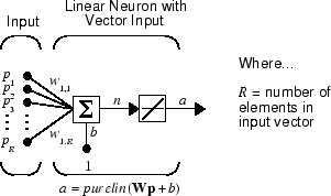
Schematic diagram showing a linear neuron with vector input. The neuron multiplies vector p by weights vector w, sums the results, and applies a bias b. The neuron then applies linear transfer function to produce output a.

This network has the same basic structure as the perceptron. The only difference is that the linear neuron uses a linear transfer function, named purelin.

A plot of the linear transfer function. The output scales linearly with the input.

The linear transfer function calculates the neuron's output by simply returning the value passed to it.

α = purelin(n) = purelin(Wp + b) = Wp + b

This neuron can be trained to learn an affine function of its inputs, or to find a linear approximation to a nonlinear function. A linear network cannot, of course, be made to perform a nonlinear computation.

Adaptive Linear Network Architecture

The ADALINE network shown below has one layer of S neurons connected to R inputs through a matrix of weights W.

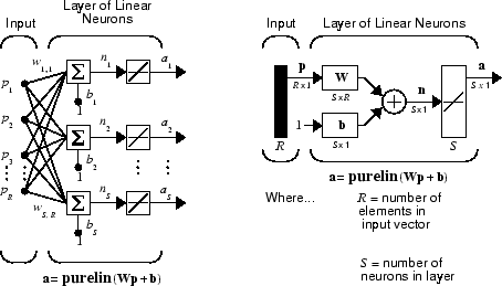
Schematic diagrams showing a layer containing S linear neurons.

This network is sometimes called a MADALINE for Many ADALINEs. Note that the figure on the right defines an S-length output vector a.

The Widrow-Hoff rule can only train single-layer linear networks. This is not much of a disadvantage, however, as single-layer linear networks are just as capable as multilayer linear networks. For every multilayer linear network, there is an equivalent single-layer linear network.

Single ADALINE (linearlayer)

Consider a single ADALINE with two inputs. The following figure shows the diagram for this network.

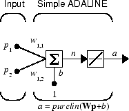
Schematic diagram showing a single ADALINE receiving a two-element vector input p. The ADALINE multiplies p by weights vector w, sums the results, and applies a bias b. The ADALINE then applies a linear transfer function to produce output a.

The weight matrix W in this case has only one row. The network output is

α = purelin(n) = purelin(Wp + b) = Wp + b

α = w_1,1p₁ + w_1,2p₂ + b

Like the perceptron, the ADALINE has a decision boundary that is determined by the input vectors for which the net input n is zero. For n = 0 the equation Wp + b = 0 specifies such a decision boundary, as shown below (adapted with thanks from [HDB96]).

Plot showing a decision boundary in the input plane.

Input vectors in the upper right gray area lead to an output greater than 0. Input vectors in the lower left white area lead to an output less than 0. Thus, the ADALINE can be used to classify objects into two categories.

However, ADALINE can classify objects in this way only when the objects are linearly separable. Thus, ADALINE has the same limitation as the perceptron.

You can create a network similar to the one shown using this command:

net = linearlayer;
net = configure(net,[0;0],[0]);

The sizes of the two arguments to configure indicate that the layer is to have two inputs and one output. Normally train does this configuration for you, but this allows us to inspect the weights before training.

The network weights and biases are set to zero, by default. You can see the current values using the commands:

W = net.IW{1,1}
W =
	 0	 0

and

b = net.b{1}
b =
	 0

You can also assign arbitrary values to the weights and bias, such as 2 and 3 for the weights and −4 for the bias:

net.IW{1,1} = [2 3];
net.b{1} = -4;

You can simulate the ADALINE for a particular input vector.

p = [5; 6];
a = sim(net,p)
a =
    24

To summarize, you can create an ADALINE network with linearlayer, adjust its elements as you want, and simulate it with sim.

Least Mean Square Error

Like the perceptron learning rule, the least mean square error (LMS) algorithm is an example of supervised training, in which the learning rule is provided with a set of examples of desired network behavior.

${p_{1}, t_{1}}, {p_{2}, t_{2}}, \dots {p_{Q}, t_{Q}}$

Here p_q is an input to the network, and t_q is the corresponding target output. As each input is applied to the network, the network output is compared to the target. The error is calculated as the difference between the target output and the network output. The goal is to minimize the average of the sum of these errors.

$m s e = \frac{1}{Q} \sum_{k = 1}^{Q} e {(k)}^{2} = \frac{1}{Q} \sum_{k = 1}^{Q} t (k) - α (k))^{2}$

The LMS algorithm adjusts the weights and biases of the ADALINE so as to minimize this mean square error.

Fortunately, the mean square error performance index for the ADALINE network is a quadratic function. Thus, the performance index will either have one global minimum, a weak minimum, or no minimum, depending on the characteristics of the input vectors. Specifically, the characteristics of the input vectors determine whether or not a unique solution exists.

You can learn more about this topic in Chapter 10 of [HDB96].

LMS Algorithm (learnwh)

Adaptive networks will use the LMS algorithm or Widrow-Hoff learning algorithm based on an approximate steepest descent procedure. Here again, adaptive linear networks are trained on examples of correct behavior.

The LMS algorithm, shown here, is discussed in detail in Linear Neural Networks.

W(k + 1) = W(k) + 2αe(k)p^T(k)

b(k + 1) = b(k) + 2αe(k)

Adaptive Filtering (adapt)

The ADALINE network, much like the perceptron, can only solve linearly separable problems. It is, however, one of the most widely used neural networks found in practical applications. Adaptive filtering is one of its major application areas.

Tapped Delay Line

You need a new component, the tapped delay line, to make full use of the ADALINE network. Such a delay line is shown in the next figure. The input signal enters from the left and passes through N-1 delays. The output of the tapped delay line (TDL) is an N-dimensional vector, made up of the input signal at the current time, the previous input signal, etc.

Schematic diagram of a tapped delay line.

Adaptive Filter

You can combine a tapped delay line with an ADALINE network to create the adaptive filter shown in the next figure.

Schematic diagram of a tapped delay line providing data to an ADALINE network. After each delay block in the delay line, the delay line provides an input to the ADALINE network. The input vector p is made up of the original signal and N progressively more delayed versions of the input signal.

The output of the filter is given by

$α (k) = p u r e l i n (W p + b) = \sum_{i = 1}^{R} w_{1,} {}_{i}α (k - i + 1) + b$

In digital signal processing, this network is referred to as a finite impulse response (FIR) filter [WiSt85]. Take a look at the code used to generate and simulate such an adaptive network.

Adaptive Filter Example

First, define a new linear network using linearlayer.

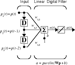
Schematic diagram of a tapped delay line providing input to a linear digital filter. The linear digital filter multiplies input p by weights vector w, sums the results, and applies a bias b. The filter then applies a linear transfer function to produce output a.

Assume that the linear layer has a single neuron with a single input and a tap delay of 0, 1, and 2 delays.

net = linearlayer([0 1 2]);
net = configure(net,0,0);

You can specify as many delays as you want, and can omit some values if you like. They must be in ascending order.

You can give the various weights and the bias values with

net.IW{1,1} = [7 8 9];
net.b{1} = [0];

Finally, define the initial values of the outputs of the delays as

pi = {1 2};

These are ordered from left to right to correspond to the delays taken from top to bottom in the figure. This concludes the setup of the network.

To set up the input, assume that the input scalars arrive in a sequence: first the value 3, then the value 4, next the value 5, and finally the value 6. You can indicate this sequence by defining the values as elements of a cell array in curly braces.

p = {3 4 5 6};

Now, you have a network and a sequence of inputs. Simulate the network to see what its output is as a function of time.

[a,pf] = sim(net,p,pi)

This simulation yields an output sequence

a
    [46]    [70]    [94]    [118]

and final values for the delay outputs of

pf
    [5]    [6]

The example is sufficiently simple that you can check it without a calculator to make sure that you understand the inputs, initial values of the delays, etc.

The network just defined can be trained with the function adapt to produce a particular output sequence. Suppose, for instance, you want the network to produce the sequence of values 10, 20, 30, 40.

t = {10 20 30 40};

You can train the defined network to do this, starting from the initial delay conditions used above.

Let the network adapt for 10 passes over the data.

for i = 1:10
    [net,y,E,pf,af] = adapt(net,p,t,pi);
end

This code returns the final weights, bias, and output sequence shown here.

wts = net.IW{1,1}
wts =
    0.5059    3.1053    5.7046
bias = net.b{1}
bias =
   -1.5993
y
y = 
    [11.8558]    [20.7735]    [29.6679]    [39.0036]

Presumably, if you ran additional passes the output sequence would have been even closer to the desired values of 10, 20, 30, and 40.

Thus, adaptive networks can be specified, simulated, and finally trained with adapt. However, the outstanding value of adaptive networks lies in their use to perform a particular function, such as prediction or noise cancelation.

Prediction Example

Suppose that you want to use an adaptive filter to predict the next value of a stationary random process, p(t). You can use the network shown in the following figure to do this prediction.

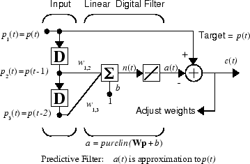
Schematic diagram of a predictive filter comprising a tapped delay line providing input to a linear digital filter.

The signal to be predicted, p(t), enters from the left into a tapped delay line. The previous two values of p(t) are available as outputs from the tapped delay line. The network uses adapt to change the weights on each time step so as to minimize the error e(t) on the far right. If this error is 0, the network output a(t) is exactly equal to p(t), and the network has done its prediction properly.

Given the autocorrelation function of the stationary random process p(t), you can calculate the error surface, the maximum learning rate, and the optimum values of the weights. Commonly, of course, you do not have detailed information about the random process, so these calculations cannot be performed. This lack does not matter to the network. After it is initialized and operating, the network adapts at each time step to minimize the error and in a relatively short time is able to predict the input p(t).

Chapter 10 of [HDB96] presents this problem, goes through the analysis, and shows the weight trajectory during training. The network finds the optimum weights on its own without any difficulty whatsoever.

Noise Cancelation Example

Consider a pilot in an airplane. When the pilot speaks into a microphone, the engine noise in the cockpit combines with the voice signal. This additional noise makes the resultant signal heard by passengers of low quality. The goal is to obtain a signal that contains the pilot's voice, but not the engine noise. You can cancel the noise with an adaptive filter if you obtain a sample of the engine noise and apply it as the input to the adaptive filter.

Schematic diagram showing an adaptive filter used to remove engine noise from a signal containing a pilot's voice and engine noise.

As the preceding figure shows, you adaptively train the neural linear network to predict the combined pilot/engine signal m from an engine signal n. The engine signal n does not tell the adaptive network anything about the pilot's voice signal contained in m. However, the engine signal n does give the network information it can use to predict the engine's contribution to the pilot/engine signal m.

The network does its best to output m adaptively. In this case, the network can only predict the engine interference noise in the pilot/engine signal m. The network error e is equal to m, the pilot/engine signal, minus the predicted contaminating engine noise signal. Thus, e contains only the pilot's voice. The linear adaptive network adaptively learns to cancel the engine noise.

Such adaptive noise canceling generally does a better job than a classical filter, because it subtracts from the signal rather than filtering it out the noise of the signal m.

Try Adaptive Noise Cancellation for an example of adaptive noise cancellation.

Multiple Neuron Adaptive Filters

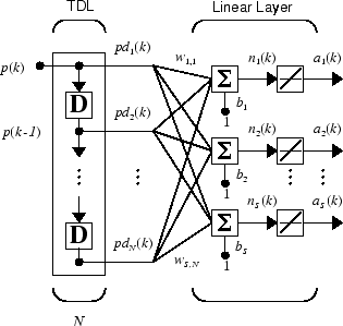
You might want to use more than one neuron in an adaptive system, so you need some additional notation. You can use a tapped delay line with S linear neurons, as shown in the next figure.

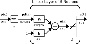
Schematic diagram of a multiple neuron adaptive filter comprising a tapped delay line providing input to a linear layer.

Alternatively, you can represent this same network in abbreviated form.

Abbreviated schematic diagram of a multiple neuron adaptive filter.

If you want to show more of the detail of the tapped delay line—and there are not too many delays—you can use the following notation:

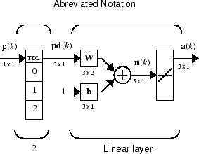
Abbreviated schematic diagram of a multiple neuron adaptive filter showing more detail of the tapped delay line.

Here, a tapped delay line sends to the weight matrix:

The current signal
The previous signal
The signal delayed before that

You could have a longer list, and some delay values could be omitted if desired. The only requirement is that the delays must appears in increasing order as they go from top to bottom.