Linear Neural Networks

The linear networks discussed in this section are similar to the perceptron, but their transfer function is linear rather than hard-limiting. This allows their outputs to take on any value, whereas the perceptron output is limited to either 0 or 1. Linear networks, like the perceptron, can only solve linearly separable problems.

Here you design a linear network that, when presented with a set of given input vectors, produces outputs of corresponding target vectors. For each input vector, you can calculate the network's output vector. The difference between an output vector and its target vector is the error. You would like to find values for the network weights and biases such that the sum of the squares of the errors is minimized or below a specific value. This problem is manageable because linear systems have a single error minimum. In most cases, you can calculate a linear network directly, such that its error is a minimum for the given input vectors and target vectors. In other cases, numerical problems prohibit direct calculation. Fortunately, you can always train the network to have a minimum error by using the least mean squares (Widrow-Hoff) algorithm.

This section introduces linearlayer, a function that creates a linear layer, and newlind, a function that designs a linear layer for a specific purpose.

Neuron Model

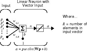
A linear neuron with R inputs is shown below.

Diagram of a linear neuron showing R inputs being multiplied by individual weights, a bias value being added, and a linear transfer function being applied to the result.

This network has the same basic structure as the perceptron. The only difference is that the linear neuron uses a linear transfer function purelin.

Plot of a linear transfer function. The output scales linearly with the input.

The linear transfer function calculates the neuron's output by simply returning the value passed to it.

$α = p u r e l i n (n) = p u r e l i n (W p + b) = W p + b$

This neuron can be trained to learn an affine function of its inputs, or to find a linear approximation to a nonlinear function. A linear network cannot, of course, be made to perform a nonlinear computation.

Network Architecture

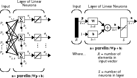
The linear network shown below has one layer of S neurons connected to R inputs through a matrix of weights W.

Network diagram of a linear network.

Note that the figure on the right defines an S-length output vector a.

A single-layer linear network is shown. However, this network is just as capable as multilayer linear networks. For every multilayer linear network, there is an equivalent single-layer linear network.

Create a Linear Neuron (linearlayer)

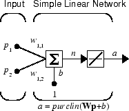
Consider a single linear neuron with two inputs. The following figure shows the diagram for this network.

Diagram of a one-neuron linear network with two inputs.

The weight matrix W in this case has only one row. The network output is

$α = p u r e l i n (n) = p u r e l i n (W p + b) = W p + b$

$α = w_{1, 1} p_{1} + w_{1, 2} p_{2} + b$

Like the perceptron, the linear network has a decision boundary that is determined by the input vectors for which the net input n is zero. For n = 0 the equation Wp + b = 0 specifies such a decision boundary, as shown below (adapted with thanks from [HDB96]).

Plot of the input space of a two-input linear network showing a decision boundary.

Input vectors in the upper right gray area lead to an output greater than 0. Input vectors in the lower left white area lead to an output less than 0. Thus, the linear network can be used to classify objects into two categories. However, it can classify in this way only if the objects are linearly separable. Thus, the linear network has the same limitation as the perceptron.

You can create this network using linearlayer, and configure its dimensions with two values so the input has two elements and the output has one.

net = linearlayer;
net = configure(net,[0;0],0);

The network weights and biases are set to zero by default. You can see the current values with the commands

W = net.IW{1,1}
W =
     0     0

and

b= net.b{1}
b =
     0

However, you can give the weights any values that you want, such as 2 and 3, respectively, with

net.IW{1,1} = [2 3];
W = net.IW{1,1}
W =
     2     3

You can set and check the bias in the same way.

net.b{1} = [-4];
b = net.b{1}
b =
     -4

You can simulate the linear network for a particular input vector. Try

p = [5;6];

You can find the network output with the function sim.

a = net(p)
a =
    24

To summarize, you can create a linear network with linearlayer, adjust its elements as you want, and simulate it with sim.

Least Mean Square Error

Like the perceptron learning rule, the least mean square error (LMS) algorithm is an example of supervised training, in which the learning rule is provided with a set of examples of desired network behavior:

${p_{1}, t_{1}}, {p_{2}, t_{2}}, \dots {p_{Q}, t_{Q}}$

Here p_q is an input to the network, and t_q is the corresponding target output. As each input is applied to the network, the network output is compared to the target. The error is calculated as the difference between the target output and the network output. The goal is to minimize the average of the sum of these errors.

$m s e = \frac{1}{Q} \sum_{k = 1}^{Q} e {(k)}^{2} = \frac{1}{Q} \sum_{k = 1}^{Q} {(t (k) - α (k))}^{2}$

The LMS algorithm adjusts the weights and biases of the linear network so as to minimize this mean square error.

Fortunately, the mean square error performance index for the linear network is a quadratic function. Thus, the performance index will either have one global minimum, a weak minimum, or no minimum, depending on the characteristics of the input vectors. Specifically, the characteristics of the input vectors determine whether or not a unique solution exists.

You can find more about this topic in Chapter 10 of [HDB96].

Linear System Design (newlind)

Unlike most other network architectures, linear networks can be designed directly if input/target vector pairs are known. You can obtain specific network values for weights and biases to minimize the mean square error by using the function newlind.

Suppose that the inputs and targets are

P = [1 2 3];
T= [2.0 4.1 5.9];

Now you can design a network.

net = newlind(P,T);

You can simulate the network behavior to check that the design was done properly.

Y = net(P)
Y =
    2.0500    4.0000    5.9500

Note that the network outputs are quite close to the desired targets.

You might try Pattern Association Showing Error Surface. It shows error surfaces for a particular problem, illustrates the design, and plots the designed solution.

You can also use the function newlind to design linear networks having delays in the input. Such networks are discussed in Linear Networks with Delays. First, however, delays must be discussed.

Linear Networks with Delays

Tapped Delay Line

You need a new component, the tapped delay line, to make full use of the linear network. Such a delay line is shown below. There the input signal enters from the left and passes through N-1 delays. The output of the tapped delay line (TDL) is an N-dimensional vector, made up of the input signal at the current time, the previous input signal, etc.

Diagram of a tapped delay line.

Linear Filter

You can combine a tapped delay line with a linear network to create the linear filter shown.

Diagram of a tapped delay line, with each delayed version of the input signal being passed to a linear layer.

The output of the filter is given by

$α (k) = p u r e l i n (W p + b) = \sum_{i = 1}^{R} w_{1, i} p (k - i + 1) + b$

The network shown is referred to in the digital signal processing field as a finite impulse response (FIR) filter [WiSt85]. Look at the code used to generate and simulate such a network.

Suppose that you want a linear layer that outputs the sequence T, given the sequence P and two initial input delay states Pi.

P = {1 2 1 3 3 2};
Pi = {1 3};
T = {5 6 4 20 7 8};

You can use newlind to design a network with delays to give the appropriate outputs for the inputs. The delay initial outputs are supplied as a third argument, as shown below.

net = newlind(P,T,Pi);

You can obtain the output of the designed network with

Y = net(P,Pi)

to give

Y = [2.7297] [10.5405] [5.0090] [14.9550] [10.7838] [5.9820]

As you can see, the network outputs are not exactly equal to the targets, but they are close and the mean square error is minimized.

LMS Algorithm (learnwh)

The LMS algorithm, or Widrow-Hoff learning algorithm, is based on an approximate steepest descent procedure. Here again, linear networks are trained on examples of correct behavior.

Widrow and Hoff had the insight that they could estimate the mean square error by using the squared error at each iteration. If you take the partial derivative of the squared error with respect to the weights and biases at the kth iteration, you have

$\frac{\partial e^{2} (k)}{\partial w_{1, j}} = 2 e (k) \frac{\partial e (k)}{\partial w_{1, j}}$

for j = 1,2,…,R and

$\frac{\partial e^{2} (k)}{\partial b} = 2 e (k) \frac{\partial e (k)}{\partial b}$

Next look at the partial derivative with respect to the error.

$\frac{\partial e (k)}{\partial w_{1, j}} = \frac{\partial [t (k) - α (k)]}{\partial w_{1, j}} = \frac{\partial}{\partial w_{1, j}} [t (k) - (W p (k) + b)]$

$\frac{\partial e (k)}{\partial w_{1, j}} = \frac{\partial}{\partial w_{1, j}} [t (k) - (\sum_{i = 1}^{R} w_{1, i} p_{i} (k) + b)]$

Here p_i(k) is the ith element of the input vector at the kth iteration.

This can be simplified to

$\frac{\partial e (k)}{\partial w_{1, j}} = - p_{j} (k)$

and

$\frac{\partial e (k)}{\partial b} = - 1$

Finally, change the weight matrix, and the bias will be

2αe(k)p(k)

and

2αe(k)

These two equations form the basis of the Widrow-Hoff (LMS) learning algorithm.

These results can be extended to the case of multiple neurons, and written in matrix form as

$\begin{array}{l} W (k + 1) = W (k) + 2 α e (k) p^{T} (k) \\ b (k + 1) = b (k) + 2 α e (k) \end{array}$

Here the error e and the bias b are vectors, and α is a learning rate. If α is large, learning occurs quickly, but if it is too large it can lead to instability and errors might even increase. To ensure stable learning, the learning rate must be less than the reciprocal of the largest eigenvalue of the correlation matrix p^Tp of the input vectors.

You might want to read some of Chapter 10 of [HDB96] for more information about the LMS algorithm and its convergence.

Fortunately, there is a toolbox function, learnwh, that does all the calculation for you. It calculates the change in weights as

dw = lr*e*p'

and the bias change as

db = lr*e

The constant 2, shown a few lines above, has been absorbed into the code learning rate lr. The function maxlinlr calculates this maximum stable learning rate lr as 0.999 * P'*P.

Type help learnwh and help maxlinlr for more details about these two functions.

Linear Classification (train)

Linear networks can be trained to perform linear classification with the function train. This function applies each vector of a set of input vectors and calculates the network weight and bias increments due to each of the inputs according to learnp. Then the network is adjusted with the sum of all these corrections. Each pass through the input vectors is called an epoch. This contrasts with adapt which adjusts weights for each input vector as it is presented.

Finally, train applies the inputs to the new network, calculates the outputs, compares them to the associated targets, and calculates a mean square error. If the error goal is met, or if the maximum number of epochs is reached, the training is stopped, and train returns the new network and a training record. Otherwise train goes through another epoch. Fortunately, the LMS algorithm converges when this procedure is executed.

A simple problem illustrates this procedure. Consider the linear network introduced earlier.

Diagram of a one-neuron linear network with two inputs.

Suppose you have the following classification problem.

${p_{1} = [\begin{array}{l} 2 \\ 2 \end{array}], t_{1} = 0} {p_{2} = [\begin{matrix} 1 \\ - 2 \end{matrix}], t_{2} = 1} {p_{3} = [\begin{matrix} - 2 \\ 2 \end{matrix}], t_{3} = 0} {p_{4} = [\begin{matrix} - 1 \\ 1 \end{matrix}], t_{4} = 1}$

Here there are four input vectors, and you want a network that produces the output corresponding to each input vector when that vector is presented.

Use train to get the weights and biases for a network that produces the correct targets for each input vector. The initial weights and bias for the new network are 0 by default. Set the error goal to 0.1 rather than accept its default of 0.

P = [2 1 -2 -1;2 -2 2 1];
T = [0 1 0 1];
net = linearlayer;
net.trainParam.goal= 0.1;
net = train(net,P,T);

The problem runs for 64 epochs, achieving a mean square error of 0.0999. The new weights and bias are

weights = net.iw{1,1}
weights =
   -0.0615   -0.2194
bias = net.b(1)
bias =
    [0.5899]

You can simulate the new network as shown below.

A = net(P)
A =
    0.0282    0.9672    0.2741    0.4320

You can also calculate the error.

err = T - sim(net,P)
err =
   -0.0282    0.0328   -0.2741    0.5680

Note that the targets are not realized exactly. The problem would have run longer in an attempt to get perfect results had a smaller error goal been chosen, but in this problem it is not possible to obtain a goal of 0. The network is limited in its capability. See Limitations and Cautions for examples of various limitations.

This example program, Training a Linear Neuron, shows the training of a linear neuron and plots the weight trajectory and error during training.

Limitations and Cautions

Linear networks can only learn linear relationships between input and output vectors. Thus, they cannot find solutions to some problems. However, even if a perfect solution does not exist, the linear network will minimize the sum of squared errors if the learning rate lr is sufficiently small. The network will find as close a solution as is possible given the linear nature of the network's architecture. This property holds because the error surface of a linear network is a multidimensional parabola. Because parabolas have only one minimum, a gradient descent algorithm (such as the LMS rule) must produce a solution at that minimum.

Linear networks have various other limitations. Some of them are discussed below.

Overdetermined Systems

Consider an overdetermined system. Suppose that you have a network to be trained with four one-element input vectors and four targets. A perfect solution to wp + b = t for each of the inputs might not exist, for there are four constraining equations, and only one weight and one bias to adjust. However, the LMS rule still minimizes the error. You might try Linear Fit of Nonlinear Problem to see how this is done.

Underdetermined Systems

Consider a single linear neuron with one input. This time, in Underdetermined Problem, train it on only one one-element input vector and its one-element target vector:

P = [1.0];
T = [0.5];

Note that while there is only one constraint arising from the single input/target pair, there are two variables, the weight and the bias. Having more variables than constraints results in an underdetermined problem with an infinite number of solutions. You can try Underdetermined Problem to explore this topic.

Linearly Dependent Vectors

Normally it is a straightforward job to determine whether or not a linear network can solve a problem. Commonly, if a linear network has at least as many degrees of freedom (S *R + S = number of weights and biases) as constraints (Q = pairs of input/target vectors), then the network can solve the problem. This is true except when the input vectors are linearly dependent and they are applied to a network without biases. In this case, as shown with the example Linearly Dependent Problem, the network cannot solve the problem with zero error. You might want to try Linearly Dependent Problem.

Too Large a Learning Rate

You can always train a linear network with the Widrow-Hoff rule to find the minimum error solution for its weights and biases, as long as the learning rate is small enough. Example Too Large a Learning Rate shows what happens when a neuron with one input and a bias is trained with a learning rate larger than that recommended by maxlinlr. The network is trained with two different learning rates to show the results of using too large a learning rate.