Code Generation for Lidar Point Cloud Segmentation Network
This example shows how to generate CUDA® MEX code for a deep learning network for lidar semantic segmentation. This example uses a pretrained SqueezeSegV2 [1] network that can segment organized lidar point clouds belonging to three classes (background, car, and truck). For information on the training procedure for the network, see Lidar Point Cloud Semantic Segmentation Using SqueezeSegV2 Deep Learning Network (Lidar Toolbox). The generated MEX code takes a point cloud as input and performs prediction on the point cloud by using the DAGNetwork object for the SqueezeSegV2 network.
Third-Party Prerequisites
Required
This example generates CUDA MEX and has the following third-party requirements.
CUDA enabled NVIDIA® GPU and compatible driver.
Optional
For non-MEX builds such as static, dynamic libraries or executables, this example has the following additional requirements.
NVIDIA toolkit.
NVIDIA cuDNN library.
NVIDIA TensorRT library.
Environment variables for the compilers and libraries. For details, see Third-Party Hardware (GPU Coder) and Setting Up the Prerequisite Products (GPU Coder).
Verify GPU Environment
To verify that the compilers and libraries for running this example are set up correctly, use the coder.checkGpuInstall (GPU Coder) function.
envCfg = coder.gpuEnvConfig('host');
envCfg.DeepLibTarget = 'cudnn';
envCfg.DeepCodegen = 1;
envCfg.Quiet = 1;
coder.checkGpuInstall(envCfg);
Segmentation Network
SqueezeSegV2 is a convolutional neural network (CNN) designed for the semantic segmentation of organized lidar point clouds. It is a deep encoder-decoder segmentation network trained on a lidar data set and imported into MATLAB® for inference. In SqueezeSegV2, the encoder subnetwork consists of convolution layers that are interspersed with max-pooling layers. This arrangement successively decreases the resolution of the input image. The decoder subnetwork consists of a series of transposed convolution layers, which successively increase the resolution of the input image. In addition, the SqueezeSegV2 network mitigates the impact of missing data by including context aggregation modules (CAMs). A CAM is a convolutional subnetwork with filterSize of value [7, 7] that aggregates contextual information from a larger receptive field, which improves the robustness of the network to missing data. The SqueezeSegV2 network in this example is trained to segment points belonging to three classes (background, car, and truck).
For more information on training a semantic segmentation network in MATLAB® by using the Mathworks® lidar dataset, see Lidar Point Cloud Semantic Segmentation Using PointSeg Deep Learning Network (Lidar Toolbox).
Download the pretrained SqueezeSegV2 Network.
net = getSqueezeSegV2Net();
Downloading pretrained SqueezeSegV2 (2 MB)...
The DAG network contains 238 layers, including convolution, ReLU, and batch normalization layers, and a focal loss output layer. To display an interactive visualization of the deep learning network architecture, use the analyzeNetwork function.
analyzeNetwork(net);
squeezesegv2_predict Entry-Point Function
The squeezesegv2_predict.m entry-point function, which is attached to this example, takes a point cloud as input and performs prediction on it by using the deep learning network saved in the SqueezeSegV2Net.mat file. The function loads the network object from the SqueezeSegV2Net.mat file into a persistent variable mynet and reuses the persistent variable in subsequent prediction calls.
type('squeezesegv2_predict.m');function out = squeezesegv2_predict(in)
%#codegen
% A persistent object mynet is used to load the DAG network object. At
% the first call to this function, the persistent object is constructed and
% setup. When the function is called subsequent times, the same object is
% reused to call predict on inputs, thus avoiding reconstructing and
% reloading the network object.
% Copyright 2020 The MathWorks, Inc.
persistent mynet;
if isempty(mynet)
mynet = coder.loadDeepLearningNetwork('SqueezeSegV2Net.mat');
end
% pass in input
out = predict(mynet,in);
Generate CUDA MEX Code
To generate CUDA MEX code for the squeezesegv2_predict.m entry-point function, create a GPU code configuration object for a MEX target and set the target language to C++. Use the coder.DeepLearningConfig (GPU Coder) function to create a CuDNN deep learning configuration object and assign it to the DeepLearningConfig property of the GPU code configuration object. Run the codegen command, specifying an input size of [64, 1024, 5]. This value corresponds to the size of the input layer of the SqueezeSegV2 network.
cfg = coder.gpuConfig('mex');
cfg.TargetLang = 'C++';
cfg.DeepLearningConfig = coder.DeepLearningConfig('cudnn');
codegen -config cfg squeezesegv2_predict -args {ones(64,1024,5,'uint8')} -report
Code generation successful: View report
To generate CUDA C++ code that takes advantage of NVIDIA TensorRT libraries, in the code, specify coder.DeepLearningConfig('tensorrt') instead of coder.DeepLearningConfig('cudnn').
For information on how to generate MEX code for deep learning networks on Intel® processors, see Code Generation for Deep Learning Networks with MKL-DNN (MATLAB Coder).
Prepare Data
Load an organized test point cloud in MATLAB®. Convert the point cloud to a five-channel image for prediction.
ptCloud = pcread('ousterLidarDrivingData.pcd');
I = pointCloudToImage(ptCloud);

% Examine converted data
whos I
  Name       Size                 Bytes  Class    Attributes

  I         64x1024x5            327680  uint8
The image has five channels. The (x,y,z) point coordinates comprise the first three channels. The fourth channel contains the lidar intensity measurement. The fifth channel contains the range information, which is computed as .
Visualize intensity channel of the image.
intensityChannel = I(:,:,4);

figure;
imshow(intensityChannel);
title('Intensity Image');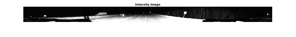
Run Generated MEX on Data
Call squeezesegv2_predict_mex on the five-channel image.
predict_scores = squeezesegv2_predict_mex(I);
The predict_scores variable is a three-dimensional matrix that has three channels corresponding to the pixel-wise prediction scores for every class. Compute the channel by using the maximum prediction score to get the pixel-wise labels
[~,argmax] = max(predict_scores,[],3);
Overlay the segmented labels on the intensity channel image and display the segmented region. Resize the segmented output and add a colorbar for better visualization.
classes = [
    "background"
    "car"
    "truck"
    ];

cmap = lidarColorMap();
SegmentedImage = labeloverlay(intensityChannel,argmax,'ColorMap',cmap);
SegmentedImage = imresize(SegmentedImage, 'Scale', [2 1], 'method', 'nearest');
figure;
imshow(SegmentedImage);

N = numel(classes);
ticks = 1/(N*2):1/N:1;
colorbar('TickLabels',cellstr(classes),'Ticks',ticks,'TickLength',0,'TickLabelInterpreter','none');
colormap(cmap)
title('Semantic Segmentation Result');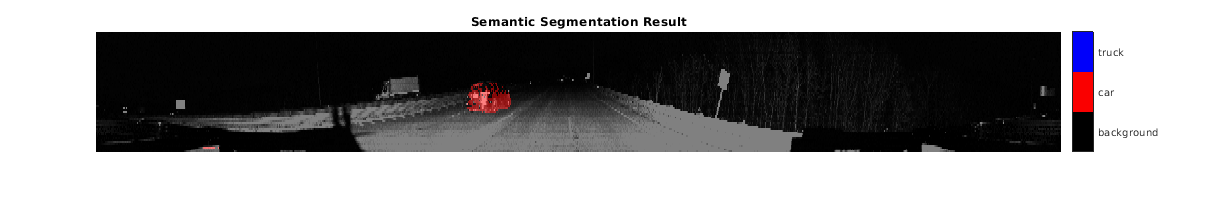
Run Generated MEX Code on Point Cloud Sequence
Read an input point cloud sequence. The sequence contains 10 organized pointCloud frames collected using an Ouster OS1 lidar sensor. The input data has a height of 64 and a width of 1024, so each pointCloud object is of size 64-by-1024.
dataFile = 'highwaySceneData.mat';

% Load data in workspace.
load(dataFile);
Setup different colors to visualize point-wise labels for different classes of interest.
% Apply the color red to cars.
carClassCar = zeros(64, 1024, 3, 'uint8');
carClassCar(:,:,1) = 255*ones(64, 1024, 'uint8');

% Apply the color blue to trucks.
truckClassColor = zeros(64, 1024, 3, 'uint8');
truckClassColor(:,:,3) = 255*ones(64, 1024, 'uint8');

% Apply the color gray to background.
backgroundClassColor = 153*ones(64, 1024, 3, 'uint8');
Set the pcplayer function properties to display the sequence and the output predictions. Read the input sequence frame by frame and detect classes of interest using the model.
xlimits = [0 120.0];
ylimits = [-80.7 80.7];
zlimits = [-8.4 27];

player = pcplayer(xlimits, ylimits, zlimits);
set(get(player.Axes,'parent'), 'units','normalized','outerposition',[0 0 1 1]);
zoom(get(player.Axes,'parent'),2);
set(player.Axes,'XColor','none','YColor','none','ZColor','none');

for i = 1 : numel(inputData)
    ptCloud = inputData{i};

    % Convert point cloud to five-channel image for prediction.
    I = pointCloudToImage(ptCloud);

    % Call squeezesegv2_predict_mex on the 5-channel image.
    predict_scores = squeezesegv2_predict_mex(I);

    % Convert the numeric output values to categorical labels.
    [~,predictedOutput] = max(predict_scores,[],3);
    predictedOutput = categorical(predictedOutput, 1:3, classes);

    % Extract the indices from labels.
    carIndices = predictedOutput == 'car';
    truckIndices = predictedOutput == 'truck';
    backgroundIndices = predictedOutput == 'background';

    % Extract a point cloud for each class.
    carPointCloud = select(ptCloud, carIndices, 'OutputSize','full');
    truckPointCloud = select(ptCloud, truckIndices, 'OutputSize','full');
    backgroundPointCloud = select(ptCloud, backgroundIndices, 'OutputSize','full');

    % Fill the colors to different classes.
    carPointCloud.Color = carClassCar;
    truckPointCloud.Color = truckClassColor;
    backgroundPointCloud.Color = backgroundClassColor;

    % Merge and add all the processed point clouds with class information.
    coloredCloud = pcmerge(carPointCloud, truckPointCloud, 0.01);
    coloredCloud = pcmerge(coloredCloud, backgroundPointCloud, 0.01);

    % View the output.
view(player, coloredCloud);
    drawnow;
end
Helper Functions
The helper functions used in this example follow.
type pointCloudToImage.mfunction image = pointCloudToImage(ptcloud) %pointCloudToImage Converts organized 3-D point cloud to 5-channel % 2-D image. image = ptcloud.Location; image(:,:,4) = ptcloud.Intensity; rangeData = iComputeRangeData(image(:,:,1),image(:,:,2),image(:,:,3)); image(:,:,5) = rangeData; % Cast to uint8. image = uint8(image); end %-------------------------------------------------------------------------- function rangeData = iComputeRangeData(xChannel,yChannel,zChannel) rangeData = sqrt(xChannel.*xChannel+yChannel.*yChannel+zChannel.*zChannel); end
type lidarColorMap.mfunction cmap = lidarColorMap() cmap = [ 0.00 0.00 0.00 % background 0.98 0.00 0.00 % car 0.00 0.00 0.98 % truck ]; end
References
[1] Wu, Bichen, Xuanyu Zhou, Sicheng Zhao, Xiangyu Yue, and Kurt Keutzer. “SqueezeSegV2: Improved Model Structure and Unsupervised Domain Adaptation for Road-Object Segmentation from a LiDAR Point Cloud.” Preprint, submitted September 22, 2018. http://arxiv.org/abs/1809.08495.