Explore ACAS Xu Neural Networks

Download ACAS Xu Neural Networks

Download the ACAS Xu neural networks [4]. The dataset contains 45 neural networks, one for each combination of nine discrete values for time until loss of vertical separation and five discrete values for the previous advisory. Each network takes the location and velocity of the ownship and the intruder ship and outputs a new advisory for the ownship: Clear-of-Conflict, Weak Left, Weak Right, Strong Left, or Strong Right.

acasXuNetworkFolder = fullfile(matlab.project.rootProject().RootFolder,".");
zipFile = matlab.internal.examples.downloadSupportFile("nnet","data/acas-xu-neural-network-dataset.zip");
filepath = fileparts(zipFile);
unzip(zipFile,acasXuNetworkFolder);

The discrete parameters characterizing the 45 different neural networks are given by:

The filenames of the networks have the form: "ACASXU_run2a_[index $$\tau$$]_[index $$a_{prev}$$]_batch_2000.onnx", reflecting the two discrete parameters. For example, "ACASXU_run2a_3_2_batch_2000.onnx" corresponds to $$\tau$$ = 1 and $$a_{prev}$$ = Weak Right.

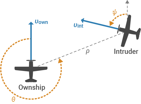
The input variables to each neural network are the positions and velocities of the ownship and intruder ship.

You can find two different versions of the ACAS Xu networks in the literature. Both definitions are equivalent in terms of network architecture and output.

However, the networks provided in the Verification of Neural Networks Competition (VNN-COM) benchmark repository [5] require shifting and rescaling of both the input and the output data. For more information, see Appendix: Data Rescaling for VNN-COMP.

The networks used in this example do not require any additional data rescaling, following the convention in Ref. [3]. Simply pass the input data to the networks using the units detailed in the above table.

Convert ONNX Models to dlnetwork Objects

The networks used in this example are saved as ONNX™ models. Convert the networks to dlnetwork objects and save them as MAT (*.mat) files by using the convertACASXuFromONNXAndSave function, which is attached to this example as a supporting file.

The final layer of the ACAS Xu network used in this example is unusual, because the predicted class corresponds to the index of the minimum output of the network, rather than the maximum output.

matFolder = fullfile(matlab.project.rootProject().RootFolder,"acas-xu-neural-network-dataset","networks-mat");
helpers.convertACASXuFromONNXAndSave(matFolder);

Importing ONNX files and converting to MAT format...
.........    ..........    ..........    ..........    ......
Import and conversion complete.

To use MATLAB® functions like scores2label, the convertACASXuFromONNXAndSave function also applies a scaling of -1 to the final fully connected layer in the network, such that the predicted class corresponds to the index of the maximum output of the network.

Make Predictions with ACAS Xu Network

Choose an ACAS Xu neural network to use based on the estimated time until loss of vertical separation and the previous advisory. To analyze different ACAS Xu neural networks, select different values for the timeUntilLossOfVerticalSeparation and previousAdvisory variables from their corresponding lists. To analyze different ACAS neural networks, select different values for these variables.

timeUntilLossOfVerticalSeparation = 1;
previousAdvisory = 1;

Load the corresponding network by using the loadACASNetwork function, which is attached to this example as a supporting file. For example, if timeUntilLossOfVerticalSeparation is 0 and previousAdvisory is Clear-of-Conflict, the function loads ACASXU_run2a_1_1_batch_2000.mat.

net = helpers.loadACASNetwork(previousAdvisory,timeUntilLossOfVerticalSeparation);

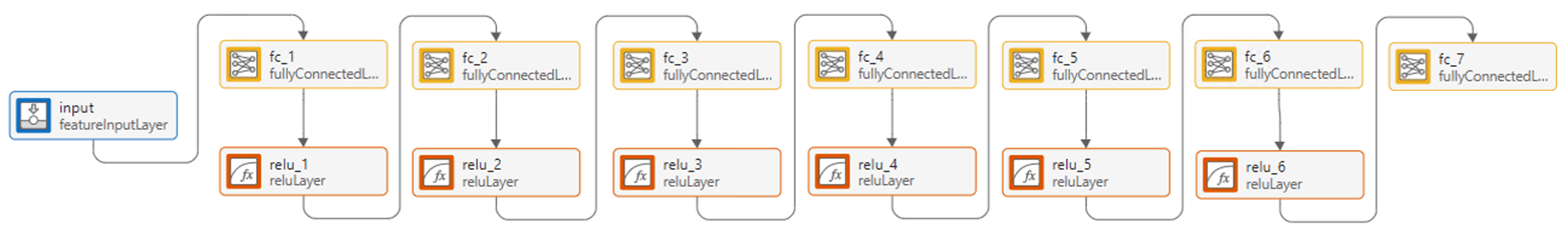
View the neural network interactively using the Deep Network Designer app:

>> deepNetworkDesigner(net)

Different configurations of the ownship and intruder require different maneuvers to avoid collision. For example, Left Abeam means that the intruder ship will collide with the ownship from the left if both aircraft stay on their current course. To avoid collision, the ownship must turn right.

First, select a different value for the configuration variable from the drop down.

configuration = 1;

Display the configuration using the displayAircraftConfiguration function, which is defined at the bottom of this example.

displayAircraftConfiguration(configuration)

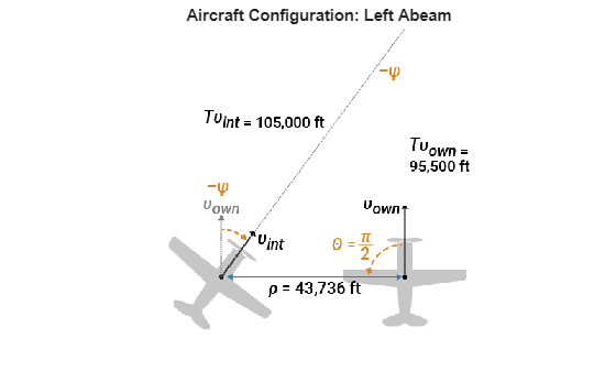
For more illustrations of the different configurations, see Fig. 5 of Ref. [2], or try setting the configuration variable to different values.

Load the dynamic variables for the chosen geometry by using the acasXuConfiguration function, which is defined at the bottom of this example.

[rho0,theta,psi,vOwn,vInt,xInt0,yInt0] = acasXuConfiguration(configuration);

In each configuration, neither aircraft changes its course. Therefore, the angles and velocities theta, psi, vOwn, and vInt do not change with time. The relative distance rho, as well as the intruder ship coordinates xInt and yInt, do change with time. The acasXuConfiguration function returns the initial values of the time dependent variables.

At the initial state of the selected configuration, the neural network advises Clear-of-Conflict, because the separation between the two aircraft is still large.

X = [rho0 theta psi vOwn vInt];
Y = predict(net,X);
advisory = scores2label(Y,helpers.classNames)

advisory = categorical
     Clear-of-Conflict 

If the two aircraft do not deviate from straight paths, the horizontal separation $\rho$ between them decreases as a linear function of time.

Assuming that the two aircraft do not change their behavior even when the advisory changes is an example of open-loop testing.

In closed-loop testing, if the predicted advisory changes, the aircraft behavior changes accordingly. Furthermore, at the next time step, the previous advisory changes and you need to use a different network. For more information on closed-loop testing, see Define and Verify AI System Requirements for ACAS Xu Neural Networks Integrated Into Simulink.

Compute the horizontal separation at several time steps between the initial time and just before the time of collision at t = 100.

t = 0:99;

% Cartesian position of ownship
xOwn = 0;
yOwn = vOwn*t;

% Cartesian position of intruder
xInt = xInt0 + vInt*sin(-psi)*t;
yInt = yInt0 + vInt*cos(-psi)*t;

% Distance between ownship and intruder
rho = sqrt((xInt - xOwn).^2 + (yInt - yOwn).^2);

Predict the advisory as a function of the horizontal separation, assuming that the previous advisory is always Clear-of-Conflict.

X = repmat([rho0,theta,psi,vOwn,vInt],[100 1]);
X(:,1) = rho;

Predict the advisory at different time steps using the predict and scores2label functions.

Y = predict(net,X);
advisory = scores2label(Y,helpers.classNames);

Plot the horizontal separation and the advisory as a function of time.

figure

yyaxis left
plot(t,rho)
ylabel("Horizontal Separation \rho (ft)",Interpreter="tex")

yyaxis right
plot(t,advisory,'.')

xlabel("Time (s)")

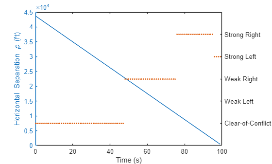
Consider an example scenario with the Left Abeam configuration and the ACASXU_run2a_1_1_batch_2000.mat network. In this scenario, as the aircraft separation decreases, the network advises Weak Right to avoid collision. When the separation decreases even further, the network advises Strong Right. Once the separation is close to zero, the network advises Strong Left.

Supporting Functions

acasXuConfiguration

The acasXuConfiguration function returns the dynamic variables for several different configurations of ownship and intruder, as detailed in Table 4 of Ref. [2]. Note that the paper differs from the example in the variables corresponding to the Right Gaining and Left Closing scenarios. To ensure that the two aircraft collide after exactly 100 s in all ten scenarios, this example uses different variables for these two scenarios.

function [rho0,theta,psi,vOwn,vInt,xInt0,yInt0] = acasXuConfiguration(scenarioIdx)
X = [43736     pi/2  -0.4296   954.6  1050  -43736        0; % Left Abeam
     43736       pi        0   462.6   900       0   -43736; % Intruder Tail Chase
     11226  -3*pi/4   0.3617   100.0   200    7096    -8699; % Right Gaining
     43736   3*pi/4  -0.5415   204.9   600  -30926   -30926; % Left Gaining
     10000     pi/4  -0.2379   362.3   300   -7069     7069; % Left Closing
     43736    -pi/2   0.6226   609.3   750   43736        0; % Right Abeam
     87472  -3*pi/8   0.7835  1145.9  1145   80814    33474; % Right Isosceles
     43736    -pi/4   0.7577   636.2   450   30926    30926; % Right Closing
     43736        0        0   497.4    60       0    43736];% Ownship Tail Chase

rho0 = X(scenarioIdx,1);
theta = X(scenarioIdx,2);
psi = X(scenarioIdx,3);
vOwn = X(scenarioIdx,4);
vInt = X(scenarioIdx,5);
xInt0 = X(scenarioIdx,6);
yInt0 = X(scenarioIdx,7);
end

displayAircraftConfiguration

The displayAircraftConfiguration function loads and displays an illustration of a selected configuration.

function displayAircraftConfiguration(scenarioIdx)
aircraftConfigurationFile = fullfile(matlab.project.rootProject().RootFolder,...
    "aircraft-configuration/","encounter-geo-closed-loop-0"+scenarioIdx+".png");
img = imread(aircraftConfigurationFile);

acasXuConfigurationNames = ["Left Abeam","Intruder Tail Chase","Right Gaining",...
    "Left Gaining","Left Closing","Right Abeam","Right Isosceles",...
    "Right Closing","Ownship Tail Chase"];

figure
imshow(img)
title("Aircraft Configuration: " + acasXuConfigurationNames(scenarioIdx))
end

Appendix: Data Rescaling for VNN-COMP

To use the ACAS Xu neural network versions in the Verification of Neural Networks Competition (VNN-COMP) benchmark repository [5], you must rescale each of the inputs and outputs of the networks.

The input rescaling is given by:

$$x_{\text{rescaled}}=\frac{x_{\text{original}}-\mu }{\sigma }$$ ,

where

The rescaling changes the permitted ranges of the input variables.

The output rescaling is given by:

$$y_{\text{rescaled}}=\frac{y_{\text{original}}-\mu }{\sigma }$$ ,

where the scale and offset are constant for each element of $$y$$: $$\mu =7.52$$ and $$\sigma =373.95$$.

References

[1] Katz, Guy. Guykatzz/ReluplexCav2017. 3 May 2017, C. 15 Jun. 2025. GitHub, https://github.com/guykatzz/ReluplexCav2017

[2] Manzanas Lopez, Diego, et al. “Evaluation of Neural Network Verification Methods for Air-to-Air Collision Avoidance.” Journal of Air Transportation, vol. 31, no. 1, Jan. 2023, pp. 1–17. DOI.org (Crossref), https://doi.org/10.2514/1.D0255.

[3] Katz, Guy, et al. “Reluplex: An Efficient SMT Solver for Verifying Deep Neural Networks.” arXiv:1702.01135, arXiv, 19 May 2017. arXiv.org, https://doi.org/10.48550/arXiv.1702.01135.

[4] “ReluplexCav2017/Nnet/ACASXU_run2a_5_9_batch_2000.Nnet at Master · Guykatzz/ReluplexCav2017.” GitHub, https://github.com/guykatzz/ReluplexCav2017/blob/master/nnet/ACASXU_run2a_5_9_batch_2000.nnet.

[5] VNN-COMP. VNN-COMP/Vnncomp2025_benchmarks. 7 May 2025, Shell. 16 Jul. 2025. GitHub, https://github.com/VNN-COMP/vnncomp2025_benchmarks.