Train Generative Adversarial Network (GAN) for Sound Synthesis
This example shows how to train and use a generative adversarial network (GAN) to generate sounds.
Introduction
In generative adversarial networks, a generator and a discriminator compete against each other to improve the generation quality.
GANs have generated significant interest in the field of audio and speech processing. Applications include text-to-speech synthesis, voice conversion, and speech enhancement.
This example trains a GAN for unsupervised synthesis of audio waveforms. The GAN in this example generates percussive sounds. The same approach can be followed to generate other types of sound, including speech.
Synthesize Audio with Pretrained GAN
Before you train a GAN from scratch, use a pretrained GAN generator to synthesize percussive sounds.
Download the pretrained generator.
loc = matlab.internal.examples.downloadSupportFile("audio","examples/PercussiveSoundGenerator.zip");
unzip(loc,pwd)
The supporting function synthesizePercussiveSound calls a pretrained network to synthesize a percussive sound sampled at 16 kHz. The synthesizePercussiveSound function is included at the end of this example.
Synthesize a percussive sound and listen to it.
synthsound = synthesizePercussiveSound();

fs = 16e3;
sound(synthsound,fs)
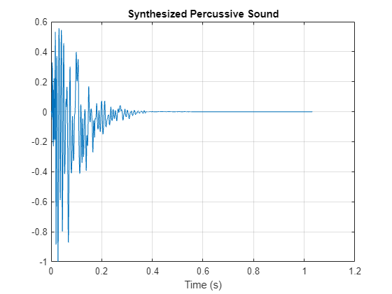
Plot the synthesized percussive sound.
t = (0:length(synthsound)-1)/fs;
plot(t,synthsound)
grid on
xlabel("Time (s)")
title("Synthesized Percussive Sound")
axis tight
You can use the percussive sounds synthesizer with other audio effects to create more complex applications. For example, you can apply reverberation to the synthesized percussive sounds.
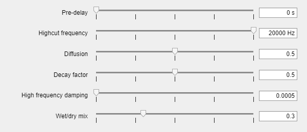
Create a reverberator (Audio Toolbox) object and open its parameter tuner UI. This UI enables you to tune the reverberator parameters as the simulation runs.
reverb = reverberator(SampleRate=fs,HighCutFrequency=12e3);
parameterTuner(reverb);
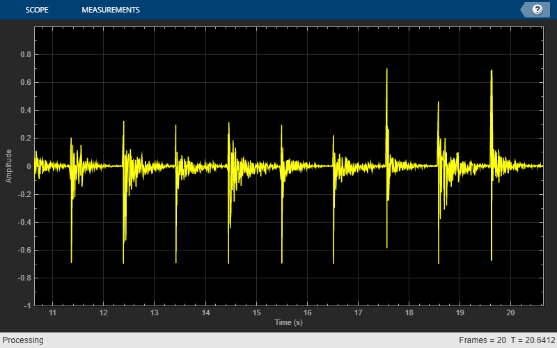
Create a timescope (DSP System Toolbox) object to visualize the percussive sounds.
ts = timescope(SampleRate=fs, ...
    TimeSpanSource="Property", ...
    TimeSpanOverrunAction="Scroll", ...
    TimeSpan=10, ...
    BufferLength=10*256*64, ...
    ShowGrid=true, ...
    YLimits=[-1 1]);
In a loop, synthesize the percussive sounds and apply reverberation. Use the parameter tuner UI to tune reverberation. If you want to run the simulation for a longer time, increase the value of the loopCount parameter.
loopCount = 20;
for ii = 1:loopCount
    synthsound = synthesizePercussiveSound;
    synthsound = reverb(gather(synthsound));
    ts(synthsound(:,1));
    soundsc(synthsound,fs)
    pause(0.5)
end
Train
Now that you have seen the pretrained percussive sounds generator in action, you can investigate the training process in detail.
A GAN is a type of deep learning network that generates data with characteristics similar to the training data.
A GAN consists of two networks that train together, a generator and a discriminator:
Generator - Given a vector or random values as input, this network generates data with the same structure as the training data. It is the generator's job to fool the discriminator.
Discriminator - Given batches of data containing observations from both the training data and the generated data, this network attempts to classify the observations as real or generated.
To maximize the performance of the generator, maximize the loss of the discriminator when given generated data. That is, the objective of the generator is to generate data that the discriminator classifies as real. To maximize the performance of the discriminator, minimize the loss of the discriminator when given batches of both real and generated data. Ideally, these strategies result in a generator that generates convincingly realistic data and a discriminator that has learned strong feature representations that are characteristic of the training data.
In this example, you train the generator to create fake time-frequency short-time Fourier transform (STFT) representations of percussive sounds. You train the discriminator to identify whether an STFT was synthesized by the generator or computed from a real audio signal. You create the real STFTs by computing the STFT of short recordings of real percussive sounds.

Download Data
Train a GAN using the Freesound One-Shot Percussive Sounds dataset [2]. Download and extract the dataset. Remove any files with licenses that prohibit commercial use.
url1 = "https://zenodo.org/record/4687854/files/one_shot_percussive_sounds.zip";
url2 = "https://zenodo.org/record/4687854/files/licenses.txt";
downloadFolder = tempdir;

percussivesoundsFolder = fullfile(downloadFolder,"one_shot_percussive_sounds");
licensefilename = fullfile(percussivesoundsFolder,"licenses.txt");
if ~datasetExists(percussivesoundsFolder)
    disp("Downloading Freesound One-Shot Percussive Sounds Dataset (112.6 MB) ...")
    unzip(url1,downloadFolder)
    websave(licensefilename,url2);
    removeRestrictiveLicense(percussivesoundsFolder,licensefilename)
end
Create an audioDatastore (Audio Toolbox) object that points to the dataset.
ads = audioDatastore(percussivesoundsFolder,IncludeSubfolders=true,OutputDataType="single");Define Preprocessing Pipeline
Generate short-time Fourier transform (STFT) data from the percussive sound signals in the datastore.
Define the STFT parameters.
fftLength = 256;
win = hann(fftLength,"periodic");
overlapLength = 128;
hopLength = numel(win) - overlapLength;
Derive the audio signal length required so that the number of hops in the STFT is equal to the number of bins in the half-sided transform. You later force the half-sided transform to have an even number of bins.
numHops = fftLength/2;
signalLength = numel(win) + (numHops-1)*hopLength;
To add a transform to the datastore to resample audio to the desired sample rate, resize the audio to the desired length, and ensure audio is mono, use the supporting function preprocessAudio.
tads = transform(ads,@(x,xinfo)preprocessAudio(x,xinfo,signalLength),IncludeInfo=true);
Add a transform to the datastore to compute the magnitude of the one-sided STFT.
tads = transform(tads,@(x){abs(stft(x,Window=win,OverlapLength=overlapLength,FrequencyRange="onesided"))});Call readall to extract the data into memory. Use a parallel pool to speed up processing if available.
STrain = readall(tads,UseParallel=canUseParallelPool);
Starting parallel pool (parpool) using the 'Processes' profile ...
21-Oct-2024 11:21:05: Job Queued. Waiting for parallel pool job with ID 1 to start ...
Connected to parallel pool with 6 workers.
The output is returned as a cell array where each element is an STFT. Concatenate the STFTs along the fourth dimension.
STrain = cat(4,STrain{:});Convert the data to the log scale to better align with human perception.
STrain = log(STrain + 1e-6);
Force the half-sided spectrum to be even.
isOddLengthHalfsided = rem(size(STrain,1),2)~=0;
if isOddLengthHalfsided
    STrain = STrain(1:end-1,:,:,:);
end
Inspect the size of the training set.
numBands = size(STrain,1)
numBands =
128
numHops = size(STrain,2)
numHops =
128
numSignals = size(STrain,4)
numSignals =
9839
Normalize training data to have zero mean and unit standard deviation.
Compute the mean and standard deviation of each frequency bin in the STFTs.
SMean = mean(STrain,[2 3 4]);
SStd = std(STrain,1,[2 3 4]);
Normalize each frequency bin.
STrain = (STrain - SMean)./SStd;
Following the approach in [1], make the data bounded by clipping the spectra to 3 standard deviations and rescaling to [-1 1].
STrain = STrain/3;
STrain = clip(STrain,-1,1);
Create an arrayDatastore to iterate over the training data.
ads = arrayDatastore(STrain,IterationDimension=4);
Create a minibatchqueue to handle batching in the training loop.
miniBatchSize = 256;
mbq = minibatchqueue(ads,MiniBatchSize=miniBatchSize,MiniBatchFormat="SSBC");
Define Generator Model
Define a network that generates STFTs of percussive sounds. The network takes 100-element latent vectors and upsamples them to a 128-by-128 arrays using a fully connected layer followed by a reshape layer and a series of transposed convolution layers with activation layers.
Specify the length of the generator input.
numLatentInputs = 100;
Specify parameters of the model. The generator architecture is defined in Table 4 of [1].
initialSize = [4,4];
filterSize = [4,4];
numFilters = [512,256,128,64,1];
numConvLayers = numel(numFilters);
numStride = [2,2];
FC1sizeControl = 1024;
FC1size = prod(initialSize)*FC1sizeControl;
Verify that the generator outputs spectrograms the same size as extracted from the real signals.
expFinalSize = [numBands,numHops]
expFinalSize = 1×2

    128    128
actFinalSize = initialSize.*numStride.^numConvLayers
actFinalSize = 1×2

    128    128
Construct the network as a sequence of layers.
layers = [
    inputLayer([numLatentInputs,1],"CB",Name="in")

    fullyConnectedLayer(FC1size,Name="FC")
    functionLayer(@(x)dlarray(reshape(stripdims(x),initialSize(1),initialSize(2),FC1sizeControl,size(x,2)),"SSCB"), ...
        Formattable=true,Acceleratable=true,Name="reshape")
    reluLayer(Name="fc_act")

    transposedConv2dLayer(filterSize,numFilters(1),Stride=numStride,Cropping="same",Name="tconv1")
    reluLayer(Name="act1")

    transposedConv2dLayer(filterSize,numFilters(2),Stride=numStride,Cropping="same",Name="tconv2")
    reluLayer(Name="act2")

    transposedConv2dLayer(filterSize,numFilters(3),Stride=numStride,Cropping="same",Name="tconv3")
    reluLayer(Name="act3")

    transposedConv2dLayer(filterSize,numFilters(4),Stride=numStride,Cropping="same",Name="tconv4")
    reluLayer(Name="act4")

    transposedConv2dLayer(filterSize,numFilters(5),Stride=numStride,Cropping="same",Name="tconv5")
    tanhLayer(Name="act5")];

netG = dlnetwork(layers);
Analyze the generator network.
analyzeNetwork(netG)

Define Discriminator Model
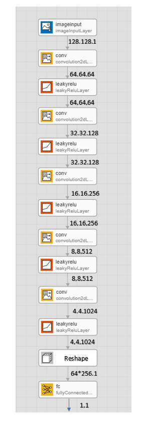
Construct a network that classifies STFTs as real or generated. The network takes 128-by-128 images and outputs a scalar prediction score using a series of convolution layers with leaky ReLU layers followed by a fully connected layer. The discriminator architecture is defined in Table 5 of [1]. Include dropout so that the discriminator does not overwhelm the generator.
dropoutProb = 0.2;
scale = 0.2;
numFiltersD = [numFilters(end-1:-1:1),FC1sizeControl];

layersDiscriminator = [
    imageInputLayer([numBands,numHops],Name="input")

    dropoutLayer(dropoutProb,Name="dropout1")

    convolution2dLayer(filterSize,numFiltersD(1),Stride=numStride,Padding="same",Name="conv1")
    leakyReluLayer(scale,Name="act1")

    convolution2dLayer(filterSize,numFiltersD(2),Stride=numStride,Padding="same",Name="conv2")
    leakyReluLayer(scale,Name="act2")

    convolution2dLayer(filterSize,numFiltersD(3),Stride=numStride,Padding="same",Name="conv3")
    leakyReluLayer(scale,Name="act3")

    dropoutLayer(dropoutProb,Name="dropout2")

    convolution2dLayer(filterSize,numFiltersD(4),Stride=numStride,Padding="same",Name="conv4")
    leakyReluLayer(scale,Name="act4")

    convolution2dLayer(filterSize,numFiltersD(5),Stride=numStride,Padding="same",Name="conv5")
    leakyReluLayer(scale,Name="act5")

    functionLayer(@(x)dlarray(reshape(stripdims(x),FC1size,size(x,4)),"CB"), ...
        Acceleratable=true,Formattable=true,Name="reshape")

    dropoutLayer(dropoutProb,Name="dropout3")

    fullyConnectedLayer(1,Name="FC")
    ];
netD = dlnetwork(layersDiscriminator );
Analyze the discriminator network.
analyzeNetwork(netD)
Define Training Options
Specify the number of epochs to train.
maxEpochs = 500;
Compute the number of iterations required to consume the data.
numIterationsPerEpoch = floor(size(STrain,4)/miniBatchSize);
Specify the options for Adam optimization. Set the learn rate of the generator and discriminator to 0.0002. For both networks, use a gradient decay factor of 0.5 and a squared gradient decay factor of 0.999.
learnRateGenerator = 0.0002;
learnRateDiscriminator = 0.0002;
gradientDecayFactor = 0.5;
squaredGradientDecayFactor = 0.999;
Train Model
Initialize the parameters for Adam.
trailingAvgGenerator = [];
trailingAvgSqGenerator = [];
trailingAvgDiscriminator = [];
trailingAvgSqDiscriminator = [];
You can set saveCheckpoints to true to save the dlnetwork to a MAT file every ten epochs. You can then use this MAT file to resume training if it is interrupted.
saveCheckpoints =  true;
true;To accelerate training, use dlaccelerate.
discriminatorGradients_acc = dlaccelerate(@discriminatorGradients);
generatorGradients_acc = dlaccelerate(@generatorGradients);
To monitor training progress, use trainingProgressMonitor.
monitor = trainingProgressMonitor( ...
   Metrics=["Generator","Discriminator"], ...
   Info=["Epoch","Iteration"], ...
   XLabel="Iteration");

groupSubPlot(monitor,Score=["Generator","Discriminator"])
Train the GAN using a custom training loop. This can take multiple hours to run.
For each epoch, shuffle the training data and loop over mini-batches of data.
iteration = 0;

for epoch = 1:maxEpochs

    % Shuffle the data
    shuffle(mbq);

    % Loop over mini-batches.
    while hasdata(mbq) && ~monitor.Stop
        iteration = iteration + 1;

        % Read mini-batch of data.
        X = next(mbq);
        thisBatchSize = size(X,finddim(X,'B'));


        % DISCRIMINATOR
        % Generate latent inputs for the generator network.
        Z = createGeneratorSeed(numLatentInputs,thisBatchSize);

        % Calculate discriminator loss and gradients
        [lossD,gradientsD,scoreD] = dlfeval(discriminatorGradients_acc,netG,netD,X,Z);

        % Update the discriminator network parameters.
        [netD,trailingAvgDiscriminator,trailingAvgSqDiscriminator] = adamupdate(netD,gradientsD, ...
            trailingAvgDiscriminator,trailingAvgSqDiscriminator,iteration, ...
            learnRateDiscriminator,gradientDecayFactor,squaredGradientDecayFactor);


        % GENERATOR
        % Generate latent inputs for the generator network.
        Z = createGeneratorSeed(numLatentInputs,thisBatchSize);

        % Calculate generator loss and gradients
        [lossG,gradientsG,scoreG] = dlfeval(generatorGradients_acc,netG,netD,Z);

        % Update the generator network parameters.
        [netG,trailingAvgGenerator,trailingAvgSqGenerator] = adamupdate(netG,gradientsG, ...
            trailingAvgGenerator,trailingAvgSqGenerator,iteration, ...
            learnRateGenerator,gradientDecayFactor,squaredGradientDecayFactor);

    end

    % Every 10 epochs, save a training snapshot to a MAT file.
    if mod(epoch,10)==0
        if saveCheckpoints
            % Save checkpoint in case training is interrupted.
            save("audiogancheckpoint.mat", ...
                "netG","netD","iteration");
        end
    end

    % Update the training progress monitor.
    recordMetrics(monitor,iteration, ...
        Generator=mean(scoreG.extractdata(),'all'), ...
        Discriminator=mean(scoreD.extractdata(),'all'));

    updateInfo(monitor,Epoch=epoch,Iteration=iteration);
    monitor.Progress = min(100*(iteration/(numIterationsPerEpoch*maxEpochs)),100);
end

Evaluate Model
Now that you have trained the network, you can investigate the synthesis process in more detail.
The trained percussive sound generator synthesizes short-time Fourier transform (STFT) matrices from input arrays of random values. An inverse STFT (ISTFT) operation converts the time-frequency STFT to a synthesized time-domain audio signal.
The generator takes vectors of random values as an input. Generate a sample input vector.
Z = createGeneratorSeed(numLatentInputs,1);
Pass the random vector to the generator to create an STFT image.
XGenerated = predict(netG,Z);
Convert the STFT dlarray to a single-precision matrix and rescale to max absolute value of 1.
Shalf = extractdata(XGenerated);
Shalf = Shalf./max(abs(Shalf),[],'all');
Revert the normalization and scaling steps used to generate the STFTs for training.
Shalf = 3*Shalf;
Shalf = (Shalf.*SStd) + SMean;
Convert the STFT from the log domain to the linear domain.
Shalf = exp(Shalf);
If the generated spectrum doesn't include the final bin of a half-sided spectrum, then add it back as zeros.
if isOddLengthHalfsided
    Shalf = cat(1,Shalf,zeros(1,size(Shalf,2)));
end
Convert the STFT from one-sided to two-sided.
if rem(fftLength,2)==0
    S = [Shalf;Shalf((end-1):-1:2,:)];
else
    S = [Shalf;Shalf(end:-1:2,:)];
end
The STFT matrix does not contain any phase information. Use stftmag2sig to estimate the signal phase and produce audio samples.
myAudio = stftmag2sig(S,fftLength, ...
    FrequencyRange="twosided", ...
    Window=win, ...
    OverlapLength=overlapLength, ...
    MaxIterations=20, ...
    Method="fgla");
myAudio = myAudio./max(abs(myAudio),[],"all");
Listen to the synthesized percussive sound.
fs = 16000;
sound(myAudio,fs)
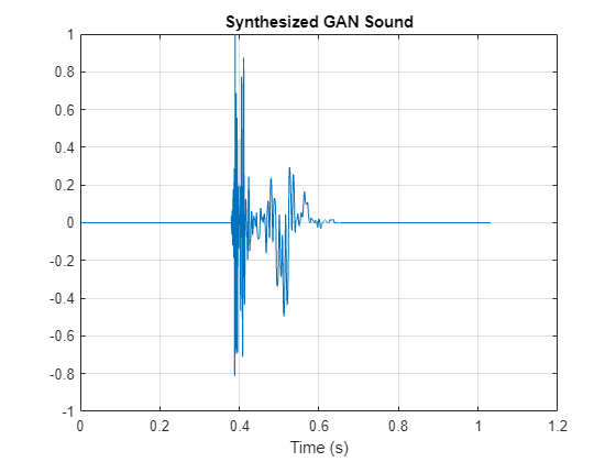
Plot the synthesized percussive sound.
t = (0:length(myAudio)-1)/fs;
plot(t,myAudio)
grid on
xlabel("Time (s)")
title("Synthesized GAN Sound")
axis tight
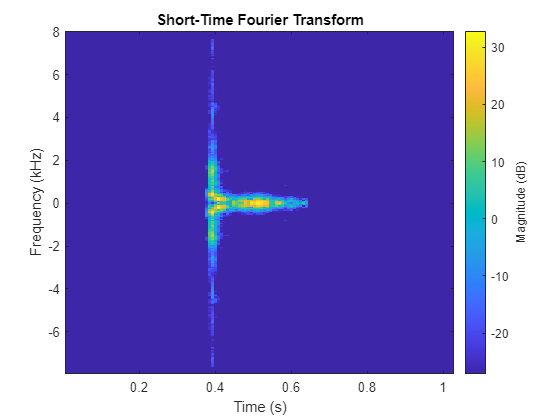
Plot the STFT of the synthesized percussive sound.
figure
stft(myAudio,fs,Window=win,OverlapLength=overlapLength);

Supporting Functions
Create Generator Seed
function Z = createGeneratorSeed(numLatentInputs,miniBatchSize)
Z = dlarray(2*(rand(numLatentInputs,miniBatchSize,"single") - 0.5 ),'CB');
if canUseGPU
    Z = gpuArray(Z);
end
end
Discriminator Gradients
function [lossD,gradientsD,scoreD] = discriminatorGradients(netG,netD,X,Z)
% Calculate the predictions for real data with the discriminator network.
X = X./max(abs(X),[],[1,2]); % ~Scale invariance
YReal  = forward(netD,X);

% Calculate the predictions for generated data with the discriminator network.
XGenerated = forward(netG,Z);
XGenerated = XGenerated./max(abs(XGenerated),[],[1,2]); % ~Scale invariance
YGenerated = forward(netD,XGenerated);

lossD = discriminatorLoss(YReal,YGenerated);

gradientsD = dlgradient(lossD,netD.Learnables);

scoreD = 0.5*(mean(sigmoid(YReal)) + mean((1 - sigmoid(YGenerated)))); % A measure of how much the discriminator was correct

end
Generator Gradients
function [lossG,gradientsG,scoreG] = generatorGradients(netG,netD,Z)

% Calculate the predictions for generated data with the discriminator network.
XGenerated = forward(netG,Z);
XGenerated = XGenerated./max(abs(XGenerated),[],[1,2]); % ~Scale invariance
YGenerated = forward(netD,XGenerated);

% Discriminator and Generator loss
lossG = generatorLoss(YGenerated);

% For each network, calculate the gradients with respect to the loss.
gradientsG = dlgradient(lossG,netG.Learnables);

scoreG = mean(sigmoid(YGenerated)); % A measure of how much the generator was fooled.
end
Discriminator Loss
function lossD = discriminatorLoss(YReal,YGenerated)
fake = dlarray(zeros(1,size(YReal,2)));
real = dlarray(ones(1,size(YReal,2)));

lossD = (mean(sigmoid_cross_entropy_with_logits(YGenerated,fake)) + ...
    mean(sigmoid_cross_entropy_with_logits(YReal,real))) / 2;
end
Generator Loss
function lossG = generatorLoss(YGenerated)
real = dlarray(ones(1,size(YGenerated,2)));
lossG = mean(sigmoid_cross_entropy_with_logits(YGenerated,real));
end
Sigmoid Cross Entropy with Logits
function out = sigmoid_cross_entropy_with_logits(x,z)
out = max(x,0) - x .* z + log(1 + exp(-abs(x)));
end
Preprocess Audio
function [out,xinfo] = preprocessAudio(in,xinfo,signalLength)
% Ensure mono
in = mean(in,2);

% Resample to 16 kHz
x = resample(in,16e3,xinfo.SampleRate);

% Force to the desired signal length
y = resize(x,signalLength,Side="both");

% Scale
out = y./max(abs(y));

end
Remove Restrictive License
function removeRestrictiveLicense(percussivesoundsFolder,licensefilename)

% Parse the licenses file that maps ids to license. Create a table to hold the info.
f = fileread(licensefilename);
K = jsondecode(f);
fns = fields(K);
T = table(Size=[numel(fns),4], ...
    VariableTypes=["string","string","string","string"], ...
    VariableNames=["ID","FileName","UserName","License"]);
for ii = 1:numel(fns)
    fn = string(K.(fns{ii}).name);
    li = string(K.(fns{ii}).license);
    id = extractAfter(string(fns{ii}),"x");
    un = string(K.(fns{ii}).username);
    T(ii,:) = {id,fn,un,li};
end

% Remove any files that prohibit commercial use. Find the file inside the
% appropriate folder, and then delete it.
unsupportedLicense = "http://creativecommons.org/licenses/by-nc/3.0/";
fileToRemove = T.ID(strcmp(T.License,unsupportedLicense));
for ii = 1:numel(fileToRemove)
    fileInfo = dir(fullfile(percussivesoundsFolder,"**",fileToRemove(ii)+".wav"));
    delete(fullfile(fileInfo.folder,fileInfo.name))
end

end
Synthesis Percussive Sound
function y = synthesizePercussiveSound

persistent pGenerator pMean pSTD
if isempty(pGenerator)
    % If the MAT file does not exist, download it
    filename = "PercussiveSoundGenerator.mat";
    load(filename,"SMean","SStd","netG");
    pMean = SMean;
    pSTD  = SStd;
    pGenerator = netG;
end

Z = createGeneratorSeed(100,1);

% Pass the random vector to the generator to create an STFT image.
XGenerated = predict(pGenerator,Z);

% Convert the STFT dlarray to a single-precision matrix.
Shalf = extractdata(XGenerated);

% Rescale.
Shalf = Shalf./max(abs(Shalf),[],'all');

% Revert the normalization and scaling steps used to generate the
% STFTs for training.
Shalf = 3*Shalf;
Shalf = (Shalf.*pSTD) + pMean;

% Convert the STFT from the log domain to the linear domain.
Shalf = exp(Shalf);

% The generated spectrum doesn't include the final bin of a
% half-sided spectrum. Add it back as zeros.
Shalf = cat(1,Shalf,zeros(1,size(Shalf,2)));

% Convert the STFT from one-sided to two-sided.
S = [Shalf;Shalf((end-1):-1:2,:)];

% The STFT matrix does not contain any phase information. Use stftmag2sig
% to estimate the signal phase and produce audio samples.
myAudio = stftmag2sig(S,256, ...
    FrequencyRange="twosided", ...
    Window=hann(256,"periodic"), ...
    OverlapLength=128, ...
    MaxIterations=20, ...
    Method="fgla");

% Rescale to a max absolute value of 1.
y = myAudio./max(abs(myAudio),[],"all");
end
Reference
[1] Donahue, C., J. McAuley, and M. Puckette. 2019. "Adversarial Audio Synthesis." ICLR.
[2] Ramires, Antonio, Pritish Chandna, Xavier Favory, Emilia Gomez, and Xavier Serra. "Neural Percussive Synthesis Parameterised by High-Level Timbral Features." ICASSP 2020 - 2020 IEEE International Conference on Acoustics, Speech and Signal Processing (ICASSP), 2020. https://doi.org/10.1109/icassp40776.2020.9053128.