Bird's-Eye Scope

Visualize sensor coverages, detections, and tracks

Description

The Bird's-Eye Scope visualizes aspects of a driving scenario or RoadRunner scenario found in your Simulink^® model.

Using the scope, you can:

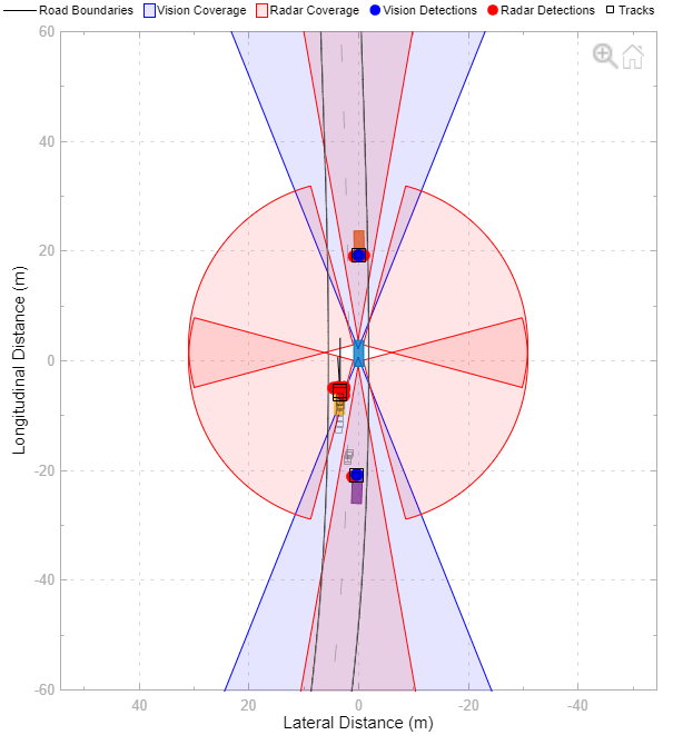
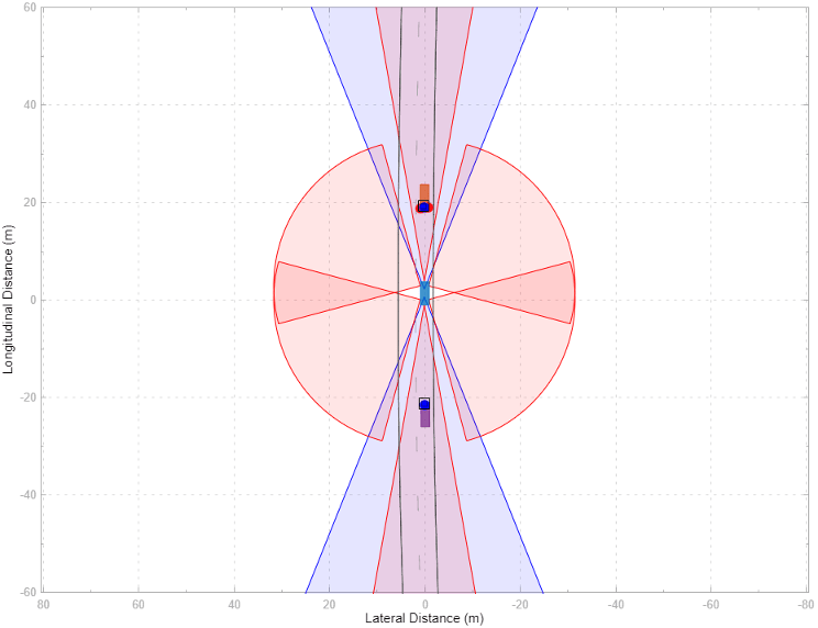
Inspect the coverage areas of radar, vision, lidar and ultrasonic sensors.
Modify sensor parameters and analyze the sensor detections of actors, road boundaries, and lane boundaries.
Analyze the tracking results of moving actors within the scenario.
Record and playback sensor detection and tracking data.

To get started, open the scope and click Find Signals. The scope updates the block diagram, finds signals representing aspects of the driving scenario, organizes the signals into groups, and displays the signals. You can then analyze the signals as you simulate, organize the signals into new groups, and modify the graphical display of the signals.

For more details about using the scope with a driving scenario, see Visualize Sensor Data and Tracks in Bird's-Eye Scope.

For more details about using the scope with a RoadRunner scenario, see Add Sensors to RoadRunner Scenario Using Simulink.

Open the Bird's-Eye Scope App

Simulink Toolstrip:

On the Simulation tab, under Review Results, click Bird's-Eye Scope.
On the Apps tab, under Signal Processing and Wireless Communications, click Bird's-Eye Scope.

Examples

Parameters

expand all

Settings > Vehicle Coordinates View

`Longitudinal axis limits` — Longitudinal axis limits
`[-60,60]` (default) | [min, max] vector

Longitudinal axis limits, specified as a [min, max] vector.

Tunable: Yes

`Lateral axis limits` — Lateral axis limits
`[-30,30]` (default) | [min, max] vector

Lateral axis limits, specified as a [min, max] vector.

Tunable: Yes

`Track position selector` — Selection matrix used to extract positions of tracked objects
`[1,0,0,0,0,0; 0,0,1,0,0,0]` (default) | 2-by-n matrix of zeros and ones

Selection matrix used to extract the positions of tracks output by the Multi-Object Tracker block. The scope extracts the positions from the state vectors of the tracks, which are stored in the State fields of the output track structures. If you specify the wrong selection, then the scope displays incorrect track positions.

Specify Track position selector as a 2-by-n matrix of zeros and ones, where n is the size of the state vectors across all tracks. These state vectors contain position, velocity, acceleration, and other state information about the tracked objects.

The default selection matrix selects track positions from a 3-D constant-velocity state vector of the form [x;vx;y;vy;z;vz]. For each track, the scope multiplies the selection matrix by the state vector to obtain the x-position and y-position, as shown here:

[1,0,0,0,0,0; 0,0,1,0,0,0] * [x;vx;y;vy;z;vz] = [x;y]

For MATLAB^® code examples illustrating this selection process, see the getTrackPositions function and multiObjectTracker object.

The formats of the state vector and corresponding selection matrix depend on the Kalman filter that the Multi-Object Tracker block uses to track objects. Suppose the Multi-Object Tracker block is initialized to use a 2-D constant-velocity linear Kalman filter, where the Filter initialization function name parameter of the block is set to the initcvkf function. For this type of filter, track states are of the form [x;vx;y;vy]. To visualize the positions of tracks output by this block, set Track position selector to [1,0,0,0; 0,0,1,0].

Tunable: No

`Track velocity selector` — Selection matrix used to extract velocities of tracked objects
`[0,1,0,0,0,0; 0,0,0,1,0,0]` (default) | 2-by-n matrix of zeros and ones

Selection matrix used to extract the velocities of tracks output by the Multi-Object Tracker block. The scope extracts the velocities from the state vectors of the tracks, which are stored in the State fields of the output track structures. If you specify the wrong selection, then the scope displays incorrect track velocities.

Specify Track velocity selector as a 2-by-n matrix of zeros and ones, where n is the size of the state vectors across all tracks. These state vectors contain position, velocity, acceleration, and other state information about the tracked objects.

The default selection matrix selects track velocities from a 3-D constant-velocity state vector of the form [x;vx;y;vy;z;vz]. For each track, the scope multiplies the selection matrix by the state vector to obtain the track velocities in the x-direction, vx, and y-direction, vy, as shown here:

[0,1,0,0,0,0; 0,0,0,1,0,0] * [x;vx;y;vy;z;vz] = [vx;vy]

For MATLAB code examples illustrating this selection process, see the getTrackVelocities function and multiObjectTracker object.

The formats of the state vector and corresponding selection matrix depend on the Kalman filter that the Multi-Object Tracker block uses to track objects. Suppose the Multi-Object Tracker block is initialized to use a 2-D constant-velocity linear Kalman filter, where the Filter initialization function name parameter of the block is set to the initcvkf function. For this type of filter, track states are of the form [x;vx;y;vy]. To visualize the velocities of tracks output by this block, set Track velocity selector to [0,1,0,0; 0,0,0,1].

Tunable: No

Settings > Global

`Display short signal names` — Display signal names without path information
`on` (default) | `off`

Select this parameter to display short signal names (signals without path information).
Clear this parameter to display long signal names (signals with path information).

Consider the signal VisionDetection within subsystem Sensor Simulation. When you select this parameter, the short name, VisionDetection, is displayed. When you clear this parameter, the long name, Sensor Simulation/VisionDetection, is displayed.

Tunable: Yes

Signal Properties (Subset Only)

`Alpha` — Transparency of coverage area
`0.1` (default) | real scalar in the range [0, 1]

Transparency of the coverage area, specified as a real scalar in the range [0, 1]. A value of 0 makes the coverage area fully transparent. A value of 1 makes the coverage area fully opaque.

This property is available only for signals in the Sensor Coverage group.

Tunable: Yes

`Velocity Scaling` — Scale factor for magnitude length of velocity vectors
`1` (default) | real scalar in the range [0, 20]

Scale factor for the magnitude length of the velocity vectors, specified as a real scalar in the range [0, 20]. The scope renders the magnitude vector value as M × Velocity Scaling, where M is the magnitude of the velocity.

This property is available only for signals in the Detections or Tracks groups.

Tunable: Yes

Limitations

General Limitations

Referenced models are not supported. To visualize signals that are within referenced models, move the output of these signals to the top-level model.
Rapid accelerator mode is not supported.
External mode and simulating a model from a generated executable is not supported.
If you initialize your model in fast restart, then after the first time you simulate, the Find Signals or Update Signals button is disabled. To enable Find Signals or Update Signals again, on the Debug tab of the Simulink toolstrip, click Fast Restart.

Scenario Reader Block Limitations

The Bird's-Eye Scope does not support visualization in a model that contains:
- More than one Scenario Reader block.
- A Scenario Reader block within a nonvirtual subsystem, such as an atomic or enabled subsystem.
- A Scenario Reader block that is configured to output actors and lane boundaries in world coordinates (Coordinate system of outputs parameter set to World Coordinates).
For Scenario Reader blocks in which you specify the ego vehicle using the Ego Vehicle input port, the ego vehicle signal must be connected directly to the block. Visualization of ego vehicle signals that are output from a nonvirtual subsystem or referenced model are not supported.

3D Simulation Block Limitations

The visualization of roads, lanes, and actors from Simulation 3D Scene Configuration blocks is not supported. If your block contains a Simulation 3D Scene Configuration block, the Bird's-Eye Scope still displays an ego vehicle, but it has default vehicle dimensions.

RoadRunner Scenario Simulation Limitations

Bird's-Eye Scope supports visualization of these lane marking types from RoadRunner scenario simulation:
- Single solid
- Double solid
- Dashed single
- Dashed solid
- Dashed double
Any other type of lane markings are not supported.

Simulation Record and Playback Limitations

The Bird's-Eye Scope app supports recording data for only a single simulation run.
Recorded simulation data is only present in the memory as long as the corresponding MATLAB instance is active.

More About

expand all

Applicable Signals

When the Bird's-Eye Scope finds signals in your model, it automatically groups signals by type. These groupings are based on the sources of the signals within the model.

Signal Group	Description	Signal Sources
Ground Truth	Road boundaries, lane markings and barriers in the scenario You cannot modify this group or any of its signals. To inspect large road networks, use the World Coordinates View window. See Vehicle and World Coordinate Views.	Scenario Reader block
Actors	Actors in the scenario, including the ego vehicle You cannot modify this group or any of its signals or subgroups. To view actors that are located away from the ego vehicle, use the World Coordinates View window. See Vehicle and World Coordinate Views.	Scenario Reader block Vision Detection Generator, Driving Radar Data Generator, and Lidar Point Cloud Generator blocks (for actor profile information only, such as the length, width, and height of actors) If actor profile information is not set or is inconsistent between blocks, the scope sets the actor profiles to the default actor profile values for each block. The profile of the ego vehicle is always set to the default profile for each block.
Sensor Coverage	Coverage areas of vision, radar, and lidar sensors, sorted into Vision, Radar, Lidar, and Ultrasonic subgroups You can modify signals in this group. You can rename or delete subgroups but not the top-level Sensor Coverage group. You can also add subgroups and move signals between subgroups. If you delete a subgroup, its signals move to the top-level Sensor Coverage group.	Vision Detection Generator block Simulation 3D Vision Detection Generator block Driving Radar Data Generator block Simulation 3D Probabilistic Radar block Lidar Point Cloud Generator block Simulation 3D Lidar block Ultrasonic Detection Generator
Detections	Detections obtained from vision, radar, and lidar sensors, sorted into Vision, Radar, Lidar, and Ultrasonic subgroups You can modify signals in this group. You can rename or delete subgroups but not the top-level Detections group. You can also add subgroups and move signals between subgroups. If you delete a subgroup, its signals move to the top-level Detections group.	Vision Detection Generator block Simulation 3D Vision Detection Generator block Driving Radar Data Generator block Lidar Point Cloud Generator block Simulation 3D Probabilistic Radar block Simulation 3D Lidar block Ultrasonic Detection Generator
Tracks	Tracks of objects in the scenario You can modify signals in this group. You can rename or delete subgroups but not the top-level Tracks group. You can also add subgroups to this group and move signals into them. If you delete a subgroup, its signals move to the top-level Tracks group.	Multi-Object Tracker block Tracker blocks in Sensor Fusion and Tracking Toolbox™ The Bird's-Eye Scope displays tracks in ego vehicle coordinates. Tracks in any other coordinate system will appear as offset in the scope.
Other Applicable Signals	Signals that the scope cannot automatically group, such as ones that combine information from multiple sensors You can modify signals in this group but you cannot add subgroups. Signals in this group do not display during simulation.	Blocks that combine or cluster signals (such as the Detection Concatenation block) Vehicle To World and World To Vehicle blocks Any blocks that create nonvirtual Simulink buses containing actor poses For details on the actor pose information required when creating these buses, see the Actors output port of the Scenario Reader block. Any blocks that create nonvirtual Simulink buses containing detections For details on the detection information required when creating these buses, see the Object Detections and Lane Detections output ports of the Vision Detection Generator block. Any blocks that create nonvirtual Simulink buses containing tracks For details on the track information required when creating these buses, see the Confirmed Tracks output port of the Multi-Object Tracker block.

To view a model that includes samples of all these signals types, see the Sensor Fusion Using Synthetic Radar and Vision Data in Simulink example.

Vehicle and World Coordinate Views

In the Bird's-Eye Scope, the default view displays the driving scenario in vehicle coordinates. During simulation, this view displays the scenario from the perspective of the ego vehicle. Use this view to inspect aspects of the scenario in the immediate vicinity of the ego vehicle.

You can also display the driving scenario in world coordinates. On the scope toolstrip, click World Coordinates to open the World Coordinates View window. Use this window to view the scenario as a whole. You can also use this view to inspect the trajectories of actors that are not in the immediate vicinity of the ego vehicle.

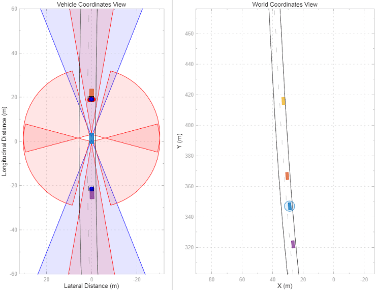
To display the roads and lanes within the World Coordinates View, click Find Signals. To display the ego vehicle and other actors in the scenario, run the simulation. This view does not display detections, tracks, sensor coverage areas, and other applicable signals. You can view these signals only in the Vehicle Coordinates View window.

Note

In the World Coordinates View window, the circle around the ego vehicle highlights the location of the vehicle in the scenario. It is not a sensor coverage area.

Tips

To find the source of a signal within the model, in the left pane of the scope, right-click a signal and select Highlight in Model.
You can show or hide signals while simulating. For example, to hide a sensor coverage, first select it from the left pane. Then, from the Properties tab, clear the Show Sensor Coverage check box.
When you reopen the scope after saving and closing a model, the scope canvas is initially blank. If you clicked Find Signals in a previous session, then click Run to run the simulation and visualize the previously found signals. The signals have the same properties from when you last saved the model. If you did not make a graphical change to the scope when you previously had it open, then the Run button is not enabled until you click Find Signals. Graphical changes include dragging signals to new groups, enabling the legend or World Coordinates View window, changing axes limits, or changing the visual properties of actors, lane markings, or sensor coverage areas.
To log and visualize new signals, click Update Signals, and then click Run to run the simulation.
If the simulation runs too quickly, you can slow it down by using simulation pacing. On the Simulation tab of the Simulink toolstrip, select Run > Simulation Pacing. Then, select the Enable pacing to slow down simulation check box and decrease the simulation time to less than the default of one second per wall clock second.
To better inspect the scenario, you can pan and zoom within the Vehicle Coordinates View and World Coordinates View windows. To return to the default display of either window, in the upper-right corner of that window, click the home button .

Version History

Introduced in R2018b

Bird's-Eye Scope

Description

Open the Bird's-Eye Scope App

Examples

Parameters

Longitudinal axis limits — Longitudinal axis limits [-60,60] (default) | [min, max] vector

Lateral axis limits — Lateral axis limits [-30,30] (default) | [min, max] vector

Track position selector — Selection matrix used to extract positions of tracked objects [1,0,0,0,0,0; 0,0,1,0,0,0] (default) | 2-by-n matrix of zeros and ones

Track velocity selector — Selection matrix used to extract velocities of tracked objects [0,1,0,0,0,0; 0,0,0,1,0,0] (default) | 2-by-n matrix of zeros and ones

Display short signal names — Display signal names without path information on (default) | off

Alpha — Transparency of coverage area 0.1 (default) | real scalar in the range [0, 1]

Velocity Scaling — Scale factor for magnitude length of velocity vectors 1 (default) | real scalar in the range [0, 20]

Limitations

More About

Applicable Signals

Vehicle and World Coordinate Views

Tips

Version History

See Also

`Longitudinal axis limits` — Longitudinal axis limits
`[-60,60]` (default) | [min, max] vector

`Lateral axis limits` — Lateral axis limits
`[-30,30]` (default) | [min, max] vector

`Track position selector` — Selection matrix used to extract positions of tracked objects
`[1,0,0,0,0,0; 0,0,1,0,0,0]` (default) | 2-by-n matrix of zeros and ones

`Track velocity selector` — Selection matrix used to extract velocities of tracked objects
`[0,1,0,0,0,0; 0,0,0,1,0,0]` (default) | 2-by-n matrix of zeros and ones

`Display short signal names` — Display signal names without path information
`on` (default) | `off`

`Alpha` — Transparency of coverage area
`0.1` (default) | real scalar in the range [0, 1]

`Velocity Scaling` — Scale factor for magnitude length of velocity vectors
`1` (default) | real scalar in the range [0, 20]