Simulate Vehicle Parking Maneuver in Driving Scenario
This example shows how to simulate a parking maneuver and generate sensor detections in a large parking lot using a cuboid driving scenario environment. This scenario and sensor simulation environment enables you to generate rare and potentially dangerous events on which to test your autonomous vehicle algorithms.
Create Scenario
The scenario used in this example contains a road, parking lot, moving vehicles, stationary vehicles, and pedestrians. The ego vehicle in this scenario contains ultrasonic sensors, which generates synthetic detections for other actors in the scene.
Define an empty scenario.
scenario = drivingScenario;
scenario.SampleTime = 0.2;
Add a two-lane, 70-meter road to the scenario.
roadCenters = [69.2 11.7 0;
              -1.1 11.5 0];
marking = [laneMarking("Solid")
           laneMarking("DoubleSolid",Color=[1 0.9 0])
           laneMarking("Solid")];
laneSpecification = lanespec(2,Width=5.925,Marking=marking);
road(scenario,roadCenters,Lanes=laneSpecification,Name="Road");
Add a second, shorter road to serve as an entrance to the parking lot.
roadCenters = [12.4 7.7 0;
               12.4 -15.8 0];
road(scenario,roadCenters,Name="Road1");
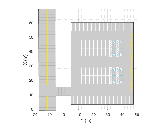
Use the parkingLot function to create a parking lot with four grids of parking spaces: one each along the top and bottom edge of the lot, and two in the middle of the lot. The parking grids along the edges contain regular parking spaces while the parking grids in the middle contain a combination of regular and accessible parking spaces. The parking lot also contains a fire lane along the right edge.
lot = parkingLot(scenario,[3 -5; 60 -5; 60 -48; 3 -48]);

% Create the parking spaces.
cars = parkingSpace;
accessible = parkingSpace(Type="Accessible");
accessibleLane = parkingSpace(Type="NoParking",MarkingColor=[1 1 1],Width=1.5);
fireLane = parkingSpace(Type="NoParking",Length=2,Width=40);

% Insert the parking spaces.
insertParkingSpaces(lot,cars,Edge=2); % Top edge
insertParkingSpaces(lot,cars,Edge=4); % Bottom edge
insertParkingSpaces(lot, ...
    [cars accessibleLane accessible accessibleLane accessible], ...
    [7 1 1 1 1],Rows=2,Position=[42 -12]);
insertParkingSpaces(lot, ...
    [cars accessibleLane accessible accessibleLane accessible], ...
    [7 1 1 1 1],Rows=2,Position=[23 -12]);
insertParkingSpaces(lot,fireLane,1,Edge=3,Offset=8); % Right edge

% Plot the scenario.
plot(scenario)
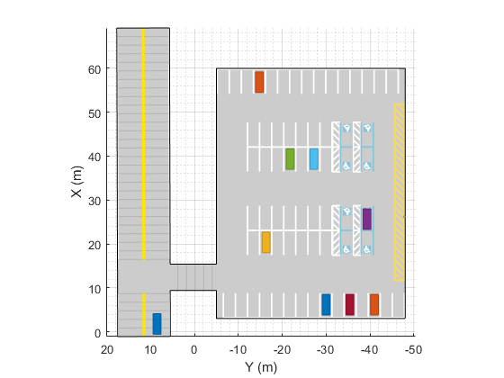
Add actors to the driving scenario. The positions and trajectories of the actors are defined in the helperAddActors supporting file.
% Add actors.
scenario = helperAddActors(scenario);

% Define ego vehicle.
ego = scenario.Actors(1);
Define Ultrasonic Sensors
In this example, you simulate an ego vehicle that has 12 ultrasonic sensors. The sensor has a maximum range of 5.5 meters, an azimuth field of view of 60 degrees, and an elevation field of view of 35 degrees. The figure in the next section displays the sensor coverage.
numUltrasonics = 12;
sensors = cell(1,numUltrasonics);
mountingLocations = [3.7 0.9 0.2; 3.7 -0.9 0.2; 3.7 0.4 0.2; 3.7 -0.4 0.2; 3.3 0.9 0.2; 3.3 -0.9 0.2; ...
    -1 0.9 0.2; -1 -0.9 0.2; -1 0.4 0.2; -1 -0.4 0.2; -0.6 0.9 0.2; -0.6 -0.9 0.2;];
mountingAngles = [45 0 0; -45 0 0; 10 0 0; -10 0 0; 80 0 0; -80 0 0; ...
    135 0 0; -135 0 0; 170 0 0; -170 0 0; 100 0 0; -100 0 0; ];
% Create all the sensors
for sndx = 1:numUltrasonics
    sensors{sndx} = ultrasonicDetectionGenerator('SensorIndex', sndx, ...
        'MountingLocation', mountingLocations(sndx,:), ...
        'MountingAngles', mountingAngles(sndx,:), ...
        'FieldOfView', [60 35]);
end

% Register actor profiles with the sensors.
profiles = actorProfiles(scenario);
for m = 1:numel(sensors)
    sensors{m}.Profiles = profiles;
end
sensorColor = [39 99 25]/255;
Visualize Scenario
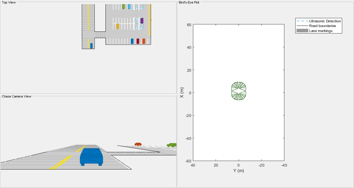
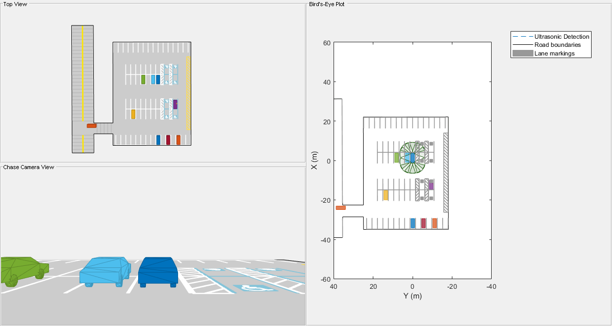
Create a display for the scenario. This display visualizes the scenario from the perspective of the ego vehicle from the top down and from behind the ego vehicle. It also displays the sensor coverage on a bird's-eye plot and returns a handle to this plot to call during simulation.
BEP = createDemoDisplay(ego,sensors,sensorColor);
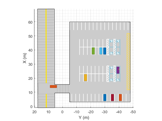
Simulate the Scenario
Use a loop to move the vehicles and call the sensor simulation.
Note that the scenario generation and sensor simulation can have different time steps. Specifying different time steps for the scenario and sensors enables you to decouple the scenario simulation from the sensor simulation. This technique is useful for modeling actor motion with high accuracy independently from the measurement rate of the sensor.
In this example, the scenario has a time step of 0.01 seconds, while the sensor detects every 0.1 seconds. The sensor returns a logical flag, isValidTime, that is true if the sensor generates detections.
while advance(scenario) && ishghandle(BEP.Parent)

    % Get scenario time
    time = scenario.SimulationTime;

    % Get position of other vehicle in ego vehicle coordinates
    poses = targetPoses(ego);

    % Simulate sensors
    detections = {};
    fovs = [];
    locations = [];
    angles = [];
    isValidTime = false;

    for sndx = 1:length(sensors)
        [sensorDets,isValidTime(sndx)] = sensors{sndx}(poses,time);
        if ~isempty(sensorDets)
            detections = [detections; sensorDets]; %#ok<*AGROW>
            fovs = [fovs sensors{sndx}.FieldOfView(1)];
            locations = [locations; sensors{sndx}.MountingLocation];
            angles = [angles; sensors{sndx}.MountingAngles];
        end
    end

    % Update bird's-eye plot
    if any(isValidTime)
        updateBEP(BEP,ego,detections,fovs,locations,angles);
    end
end
Summary
This example showed how to generate a scenario containing a parking lot, simulate sensor detections, and use these detections to detect vehicles and pedestrians in the parking lot.
You can try to modify the parking lot or add or remove vehicles. You can also try to add, remove, or modify the sensors on the ego vehicle.
Supporting Functions
createDemoDisplay
This function creates a three-pane display:
Top-left pane — A top view that follows the ego vehicle.
Bottom-left pane — A chase-camera view that follows the ego vehicle.
Right pane — A
birdsEyePlot
function BEP = createDemoDisplay(egoCar,sensors,sensorColor)
    % Make a figure
    hFigure = figure(Position=[0 0 1200 640],Name="Parking Maneuver Scenario");
    movegui(hFigure,[0 -1]); % Moves figure left and a little down from the top

    % Add a car plot that follows the ego vehicle from behind
    hCarViewPanel = uipanel(hFigure,Position=[0 0 0.5 0.5],Title="Chase Camera View");
    hCarPlot = axes(hCarViewPanel);
    chasePlot(egoCar,Parent=hCarPlot,Meshes="on");

    % Add a car plot that follows the ego vehicle from a top view
    hTopViewPanel = uipanel(hFigure,Position=[0 0.5 0.5 0.5],Title="Top View");
    hCarPlot = axes(hTopViewPanel);
    chasePlot(egoCar,Parent=hCarPlot,ViewHeight=130,ViewLocation=[0 0],ViewPitch=90);

    % Add pane for bird's-eye plot
    hBEVPanel = uipanel(hFigure,Position=[0.5 0 0.5 1],Title="Bird's-Eye Plot");

    % Create bird's-eye plot for the ego vehicle and sensor coverage
    hBEVPlot = axes(hBEVPanel);
    frontBackLim = 60;
    BEP = birdsEyePlot(Parent=hBEVPlot,Xlimits=[-frontBackLim frontBackLim],Ylimits=[-35 35]);

    % Plot the coverage area for ultrasonic
    for sndx = 1:length(sensors)
        cap = coverageAreaPlotter(BEP,FaceColor=sensorColor,EdgeColor=sensorColor);
        plotCoverageArea(cap,sensors{sndx}.MountingLocation(1:2), ...
            sensors{sndx}.DetectionRange(3),sensors{sndx}.MountingAngles(1),sensors{sndx}.FieldOfView(1));
    end

    % Combine all ultrasonic detections into one entry and store it for later update
    rangeDetectionPlotter(BEP,DisplayName="Ultrasonic Detection",LineStyle='--');

    % Add road borders to plot
    laneBoundaryPlotter(BEP,DisplayName="Road boundaries");

    % Add lane markings to plot
    laneMarkingPlotter(BEP,DisplayName="Lane markings");

    axis(BEP.Parent,"equal");
    xlim(BEP.Parent,[-frontBackLim frontBackLim]);
    ylim(BEP.Parent,[-40 40]);

    % Add an outline plotter for ground truth
    outlinePlotter(BEP,Tag="Ground truth");
end
updateBEP
This function updates the bird's-eye plot with road boundaries, ranges, and tracks.
function updateBEP(BEP,ego,detections,fovs,locations,angles)
    % Update road boundaries and their display
    [lmv,lmf] = laneMarkingVertices(ego);
    plotLaneMarking(findPlotter(BEP,DisplayName="Lane markings"),lmv,lmf);

    % Update parking lot boundaries and markings and their display
    [plmv,plmf] = parkingLaneMarkingVertices(ego);
    plotParkingLaneMarking(findPlotter(BEP,DisplayName="Lane markings"),plmv,plmf);

    % Update ground truth data
    [position,yaw,length,width,originOffset,color] = targetOutlines(ego);
    plotOutline(findPlotter(BEP,Tag="Ground truth"),position,yaw,length,width, ...
        OriginOffset=originOffset,Color=color);

    % Update road boundaries
    rbs = roadBoundaries(ego);
    plotLaneBoundary(findPlotter(BEP,DisplayName="Road boundaries"),rbs);

    % Prepare and update detections display
    N = numel(detections);
    detRanges = zeros(N,1);
    for i = 1:N
        detRanges(i,:) = detections{i}.Measurement(1);
    end
    if ~isempty(detRanges)
        plotRangeDetection(findPlotter(BEP,DisplayName="Ultrasonic Detection"), detRanges, fovs, locations, angles);
    end
end
See Also
drivingScenario | parkingSpace | insertParkingSpaces | birdsEyePlot