BilevelMeasurementsConfiguration
Description
Use the BilevelMeasurementsConfiguration object to measure
transitions, aberrations, and cycles of bilevel signals. You can also specify the bilevel
settings such as high-state level, low-state level, state-level tolerance, upper-reference
level, mid-reference level, and lower-reference level.
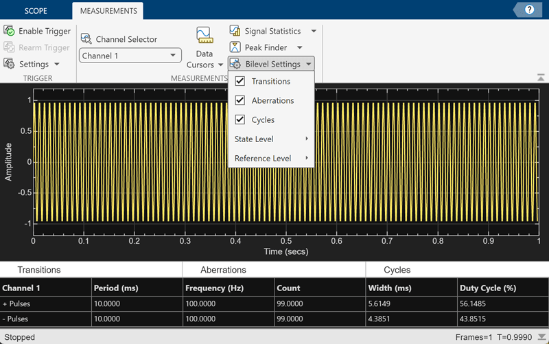
You can control bilevel measurements from the toolstrip or from the command line. To modify bilevel measurements from the toolstrip, in the Measurements tab, click Bilevel Settings and select the measurements you want to display. A panel appears at the bottom of the Time Scope window showing all the measurements you enabled.


Creation
Description
bilevelMeas = BilevelMeasurementsConfiguration() creates a
bilevel measurements configuration object.
Properties
All properties are tunable.
Automatic detection of high- and low-state levels, specified as
true or false. Set this property to
true so that the scope automatically detects high- and low-state
levels in the bilevel waveform. When you set this property to false,
you can specify values for the high- and low- state levels manually using the
HighStateLevel and LowStateLevel
properties.
Scope Window Use
On the Measurements tab, in the Measurements section, click Bilevel Settings. Under State Level, and select Auto State Level.
Data Types: logical
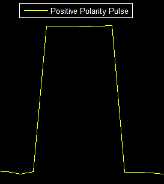
High-state level, specified as a nonnegative scalar. The high-state level denotes a positive polarity.
If the initial transition of a pulse is positive-going, the pulse has positive polarity. The terminating state of a positive-polarity (positive-going) pulse is more positive than the originating state.
This figure shows a positive-polarity pulse.
Dependency
To enable this property, set AutoStateLevel to
false.
Scope Window Use
On the Measurements tab, in the Measurements section, click Bilevel Settings. Under State Level, clear Auto State Level and specify a nonnegative scalar in the High box.
Data Types: double
High-state level, specified as a nonnegative scalar. The low-state level denotes a negative polarity.
If the initial transition of a pulse is negative-going, the pulse has negative polarity. The terminating state of a negative-polarity (negative-going) pulse is more negative than the originating state.
This figure shows a negative-polarity pulse.

Dependency
To enable this property, set AutoStateLevel to
false.
Scope Window Use
On the Measurements tab, in the Measurements section, click Bilevel Settings. Under State Level, clear Auto State Level and specify a nonnegative scalar in the Low box.
Data Types: double
Tolerance level of the state, specified as a positive scalar in the range (0 100).
This value determines how much a signal can deviate from the low- or high-state level before it is considered to be outside that state. Specify this value as a percentage of the difference between the high- and low-state levels. For more details, see State-Level Tolerances.
Scope Window Use
On the Measurements tab, in the Measurements section, click Bilevel Settings. Under State Level, specify a positive scalar less than 100 in the State Level Tol. (%) box.
Data Types: double
Upper-reference level, specified as a positive scalar in the range (0 100). The scope uses the upper-reference level to compute the start of a fall time or the end of a rise time. Specify this value as a percentage of the difference between the high- and low-state levels.
If S1 is the low-state level, S2 is the high-state level, and U is the upper-reference level, the waveform value corresponding to the upper-reference level is
Scope Window Use
On the Measurements tab, in the Measurements section, click Bilevel Settings. Under Reference Level, specify a positive scalar less than 100 in the Upper Ref. Level (%) box.
Data Types: double
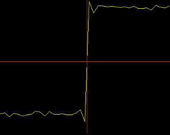
Mid-reference level, specified as a positive scalar in the range (0 100). The scope uses the mid-reference level to determine when a transition occurs. Specify this value as a percentage of the difference between the high- and low-state levels.
The mid-reference level in a bilevel waveform with low-state level S1 and high-state level S2 is
This figure shows the mid-reference level as a horizontal line, and shows its corresponding mid-reference level instant as a vertical line.
Scope Window Use
On the Measurements tab, in the Measurements section, click Bilevel Settings. Under Reference Level, specify a positive scalar less than 100 in the Mid Ref. Level (%) box.
Data Types: double
Lower-reference level, specified as a positive scalar in the range (0 100). The scope uses the lower-reference level to compute the end of a fall time or the start of a rise time. Specify this value as a percentage of the difference between the high- and low-state levels.
If S1 is the low-state level, S2 is the high-state level, and L is the lower-reference level, the waveform value corresponding to the lower-reference level is
Scope Window Use
On the Measurements tab, in the Measurements section, click Bilevel Settings. Under Reference Level, specify a positive scalar less than 100 in the Lower Ref. Level (%) box.
Data Types: double
Time duration over which the scope searches for a settling time, specified as a positive scalar in seconds.
Scope Window Use
On the Measurements tab, in the Measurements section, click Bilevel Settings. Under Reference Level, specify a positive scalar in the Settle Seek (s) box.
Data Types: double
Enable transition measurements, specified as true or
false. For more information on the transition measurements that the
scope displays, see Transitions Pane (Simulink).
Scope Window Use
On the Measurements tab, in the Measurements section, click Bilevel Settings and select Transitions. A Transitions pane opens at the bottom of the Time Scope window to show the transition measurements.
Data Types: logical
Enable aberration measurements, specified as true or
false. Aberration measurements include distortion and damping
measurements such as preshoot, overshoot, and undershoot. For more information on the
aberration measurements that the scope displays, see Aberrations Pane (Simulink).
Scope Window Use
On the Measurements tab, in the Measurements section, click Bilevel Settings and select Aberrations. An Aberrations pane opens at the bottom of the Time Scope window to show the aberration measurements.
Data Types: logical
Enable cycle measurements, specified as true or
false. These measurements are related to repetitions or trends in
the displayed portion of the input signal. For more information on the cycle
measurements, see Cycles Pane (Simulink).
Scope Window Use
On the Measurements tab, in the Measurements section, click Bilevel Settings and select Cycles. A Cycles pane opens at the bottom of the Time Scope window to show the cycle measurements.
Data Types: logical
Examples
Create a sine wave and view it in the Time Scope. Programmatically compute the bilevel measurements related to signal transitions, aberrations, and cycles.
The timescope object requires one of these products:
DSP System Toolbox™
Navigation Toolbox™
Sensor Fusion and Tracking Toolbox™
Initialization
Create the input sine wave using the sin function. Create a timescope MATLAB® object to display the signal. Set the TimeSpan property to 1 second.
f = 100;
fs = 1000;
swv = sin(2.*pi.*f.*(0:1/fs:1-1/fs)).';
scope = timescope(SampleRate=fs,...
    TimeSpanSource="property",...
    TimeSpan=1);
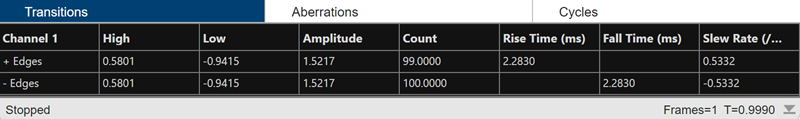
Transition Measurements
Enable the scope to show transition measurements programmatically by setting the ShowTransitions property to true. Display the sine wave in the scope.
Transition measurements such as rise time, fall time, and slew rate appear in the Transitions pane at the bottom of the scope.
scope.BilevelMeasurements.ShowTransitions = true;
scope(swv);
release(scope);

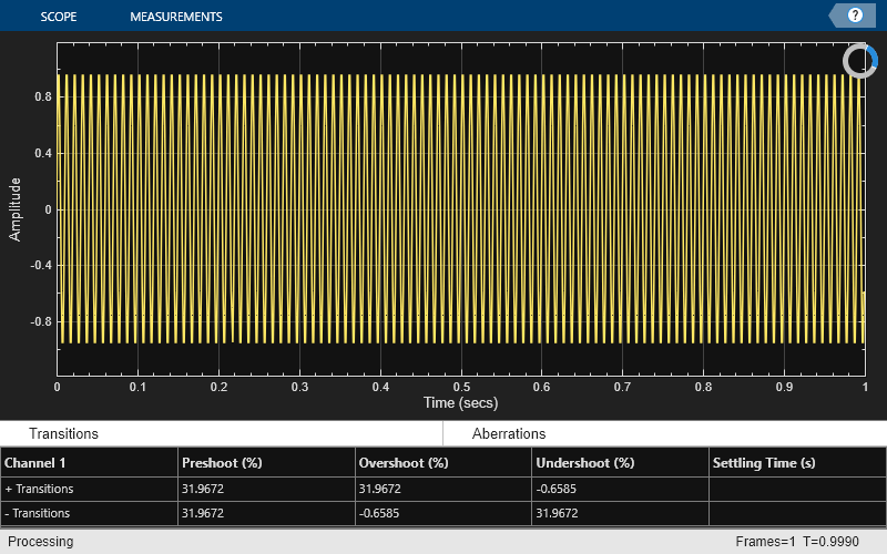
Aberration Measurements
Enable the scope to show aberration measurements programmatically by setting the ShowAberrations property to true. Display the sine wave in the scope.
Aberration measurements such as preshoot, overshoot, undershoot, and settling time appear in the Aberrations pane at the bottom of the scope.
scope.BilevelMeasurements.ShowAberrations = true;
scope(swv);
release(scope);
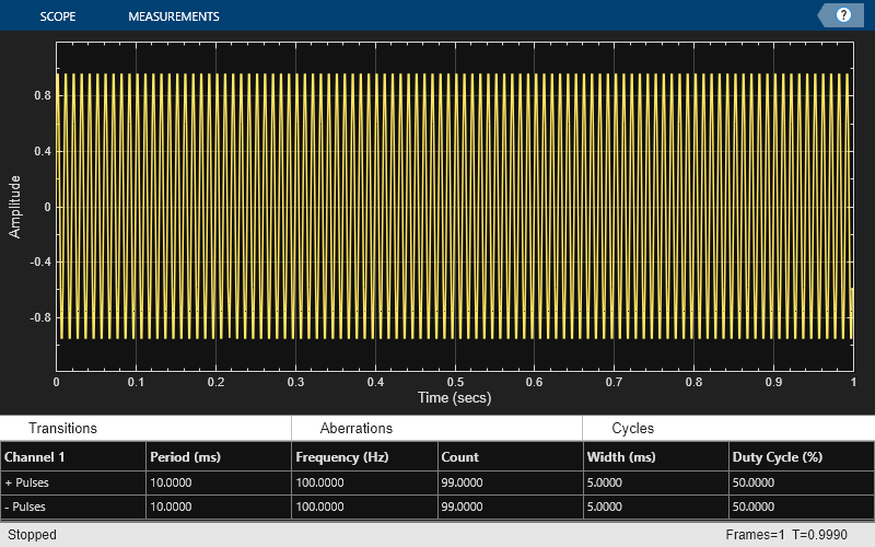
Cycle Measurements
Enable the scope to show cycles measurements programmatically by setting the ShowCycles property to true. Display the sine wave in the scope.
Cycle measurements such as period, frequency, pulse width, and duty cycle appear in the Cycles pane at the bottom of the scope.
scope.BilevelMeasurements.ShowCycles = true;
scope(swv);
release(scope);
More About
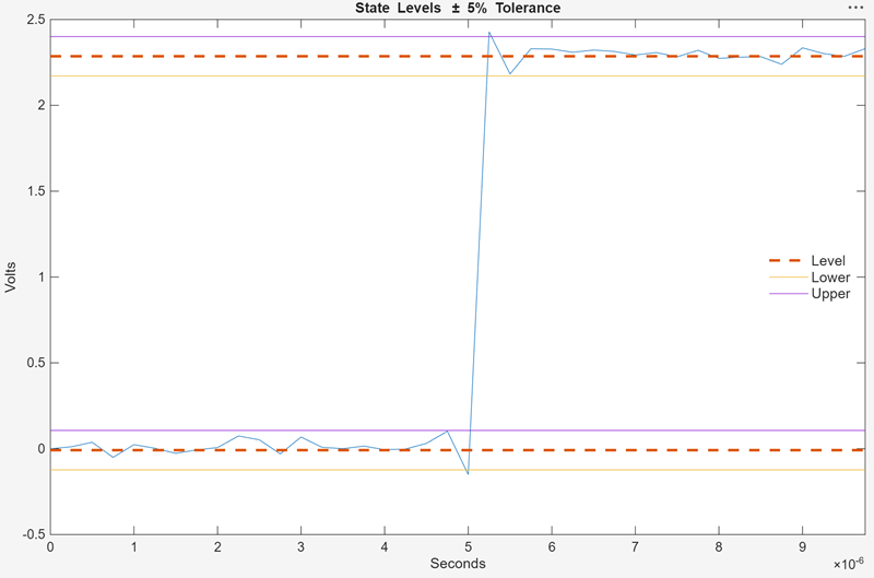
You can specify lower- and upper-state boundaries for each state level. Define the boundaries as the state level plus or minus a scalar multiple of the difference between the high state and the low state. To provide a useful tolerance region, specify the scalar as a small number such as 2/100 or 3/100. In general, the α% region for the low state is defined as:
where S1 is the low-state level and S2 is the high-state level. Replace the first term in the equation with S2 to obtain the α% tolerance region for the high state.
The figure shows lower and upper 5% state boundaries (tolerance regions) for a positive-polarity bilevel waveform. The thick dashed lines indicate the estimated state levels.
Version History
Introduced in R2022a