dsp.SineWave

Generate discrete sine wave

Description

The dsp.SineWave System object™ generates a real or complex, multichannel sinusoidal signal with independent amplitude, frequency, and phase in each output channel.

For both real and complex sinusoids, the Amplitude, Frequency, and PhaseOffset properties can be scalars or length-N vectors, where N is the number of channels in the output. When you specify at least one of these properties as a length-N vector, scalar values specified for the other properties are applied to each of the N channels.

The dsp.SineWave object and the sin function both generate a discrete sine wave signal. However, the object can process large streams of real-time data and handle system states automatically. The function performs one-time computations on data that is readily available and cannot handle system states. For a comparison between the two, see System Objects vs MATLAB Functions.

To generate a discrete-time sinusoidal signal:

Create the dsp.SineWave object and set its properties.
Call the object with arguments, as if it were a function.

To learn more about how System objects work, see What Are System Objects?

Creation

Syntax

sine = dsp.SineWave

sine = dsp.SineWave(Name,Value)

sine = dsp.SineWave(amp,freq,phase,Name,Value)

Description

sine = dsp.SineWave creates a sine wave object that generates a real-valued sinusoid with an amplitude of 1, a frequency of 100 Hz, and a phase offset of 0. By default, the sine wave object generates only one sample.

sine = dsp.SineWave(Name,Value) creates a sine wave object with each specified property set to the specified value. Enclose each property name in single quotes.

Example: sine = dsp.SineWave('Amplitude',2);

sine = dsp.SineWave(amp,freq,phase,Name,Value) creates a sine wave object with the Amplitude property set to amp, Frequency property set to freq, PhaseOffset property set to phase, and any other specified properties set to the specified values.

example

Properties

expand all

Unless otherwise indicated, properties are nontunable, which means you cannot change their values after calling the object. Objects lock when you call them, and the release function unlocks them.

If a property is tunable, you can change its value at any time.

For more information on changing property values, see System Design in MATLAB Using System Objects.

`Amplitude` — Amplitude of sine wave
`1` (default) | scalar | vector

Amplitude of the sine wave, specified as one of the following:

scalar –– A scalar applies to all channels.
vector –– A length-N vector contains the amplitudes of the sine waves in each of the N output channels. The vector length must be the same as that specified for the Frequency and PhaseOffset properties.

Tunable: Yes

Dependencies

This property is tunable only when you set Method to either 'Trigonometric function' or 'Differential'.

`Frequency` — Frequency of sine wave
`100` (default) | scalar | vector

Frequency of the sine wave in Hz, specified as one of the following:

scalar –– A scalar applies to all channels.
vector –– A length-N vector contains the frequencies of the sine waves in each of the N output channels. The vector length must be the same as that specified for the Amplitude and PhaseOffset properties.

`PhaseOffset` — Phase offset of sine wave
`0` (default) | scalar | vector

Phase offset of the sine wave in radians, specified as one of the following:

scalar –– A scalar applies to all channels.
vector –– A length-N vector contains the phase offsets of the sine waves in each of the N output channels. The vector length must be the same as that specified for the Amplitude and Frequency properties.

`ComplexOutput` — Flag that indicates whether waveform is real or complex
`false` (default) | `true`

Flag that indicates whether the waveform is real or complex, specified as either:

false –– The waveform output is real.
true –– The waveform output is complex.

`Method` — Method used to generate sinusoids
`'Trigonometric function'` (default) | `'Table lookup'` | `'Differential'`

Method used to generate sinusoids, specified as one of the following:

'Trigonometric function' –– The object computes the sinusoid by sampling the continuous-time function.
'Table lookup' –– The object precomputes the unique samples of every output sinusoid at the start of the simulation, and recalls the samples from memory as needed.
'Differential' –– The object uses an incremental algorithm. This algorithm computes the output samples based on the output values computed at the previous sample time and precomputed update terms.

`TableOptimization` — Optimize table of sine values for speed or memory
`'Speed'` (default) | `'Memory'`

Optimize table of sine values for speed or memory, specified as either:

'Speed' –– The table contains k elements, where k is the number of input samples in one full period of the sine wave. The period of each sinusoid must be an integer multiple of 1/Fs, where Fs is the value of the SampleRate property value. That is, each element of the Frequency property must be of the form Fs/m, where m is an integer greater than 1.
'Memory' –– The table contains k/4 elements.

Dependencies

This property applies only when you set the Method property to 'Table lookup'.

`SampleRate` — Sample rate of output signal
`1000` (default) | positive scalar

Sample rate of output signal in Hz, specified as a positive scalar.

Example: 44100

Example: 22050

`SamplesPerFrame` — Number of samples per frame
`1` (default) | positive integer

Number of consecutive samples from each sinusoid to buffer into the output frame, specified as a positive integer.

Example: 1000

Example: 5000

`OutputDataType` — Data type of the sine wave output
`'double'` (default) | `'single'` | `'Custom'`

Data type of the sine wave output, specified as 'double', 'single', or 'Custom'.

Fixed-Point Properties

`CustomOutputDataType` — Output word and fraction lengths
`numerictype([],16)` (default) | `numerictype([],32,30)`

Output word and fraction lengths, specified as an autosigned numeric type with a word length of 16.

Example: numerictype([],32,30)

Example: numerictype([],16,15)

Dependencies

This property applies only when you set the Method property to 'Table lookup' and the OutputDataType property to 'Custom'.

Usage

Syntax

sineOut = sine()

Description

sineOut = sine() creates the sine wave output, sineOut.

example

Output Arguments

expand all

`sineOut` — Sine wave output
vector | matrix

Sine wave output, returned as a vector or matrix. The SamplesPerFrame property determines the number of rows in the output matrix. If the Frequency or the PhaseOffset property is a vector, the length of the vector determines the number of columns (channels) in the output matrix. If the Frequency or the PhaseOffset properties is a scalar, then the number of channels in the output matrix is 1.

The OutputDataType property sets the data type of the output.

Data Types: single | double | fi

Object Functions

To use an object function, specify the System object as the first input argument. For example, to release system resources of a System object named obj, use this syntax:

release(obj)

expand all

Common to All System Objects

`step`	Run System object algorithm
`release`	Release resources and allow changes to System object property values and input characteristics
`reset`	Reset internal states of System object

Examples

collapse all

Generate a Sine Wave Signal

Open Live Script

Generate a sine wave with an amplitude of 2, frequency of 10 Hz, and an initial phase of 0.

sine1 = dsp.SineWave(2,10);
sine1.SamplesPerFrame = 1000;
y = sine1();
plot(y)

Figure contains an axes object. The axes object contains an object of type line.

Generate two sine waves offset by a phase of pi/2 radians.

sine2 = dsp.SineWave;
sine2.Frequency = 10;
sine2.PhaseOffset = [0 pi/2];
sine2.SamplesPerFrame = 1000;
y = sine2();
plot(y)

Figure contains an axes object. The axes object contains 2 objects of type line.

Filter Frames of a Noisy Sine Wave Signal in MATLAB

Open Live Script

This example shows how to lowpass filter a noisy signal in MATLAB® and visualize the original and filtered signals using a spectrum analyzer. For a Simulink® version of this example, see Filter Frames of a Noisy Sine Wave Signal in Simulink.

Specify Signal Source

The input signal is the sum of two sine waves with frequencies of 1 kHz and 10 kHz. The sampling frequency is 44.1 kHz.

Sine1 = dsp.SineWave('Frequency',1e3,'SampleRate',44.1e3);
Sine2 = dsp.SineWave('Frequency',10e3,'SampleRate',44.1e3);

Create Lowpass Filter

The lowpass FIR filter, dsp.LowpassFilter, designs a minimum-order FIR lowpass filter using the generalized Remez FIR filter design algorithm. Set the passband frequency to 5000 Hz and the stopband frequency to 8000 Hz. The passband ripple is 0.1 dB and the stopband attenuation is 80 dB.

FIRLowPass = dsp.LowpassFilter('PassbandFrequency',5000,...
    'StopbandFrequency',8000);

Create Spectrum Analyzer

Set up the spectrum analyzer to compare the power spectra of the original and filtered signals. The spectrum units are dBm.

SpecAna = spectrumAnalyzer('PlotAsTwoSidedSpectrum',false,...
    'SampleRate',Sine1.SampleRate,...
    'ShowLegend',true, ...
    'YLimits',[-145,45]);

SpecAna.ChannelNames = {'Original noisy signal',...
    'Lowpass filtered signal'};

Specify Samples per Frame

This example uses frame-based processing, where data is processed one frame at a time. Each frame of data contains sequential samples from an independent channel. Frame-based processing is advantageous for many signal processing applications because you can process multiple samples at once. By buffering your data into frames and processing multisample frames of data, you can improve the computational time of your signal processing algorithms. Set the number of samples per frame to 4000.

Sine1.SamplesPerFrame = 4000;
Sine2.SamplesPerFrame = 4000;

Filter the Noisy Sine Wave Signal

Add zero-mean white Gaussian noise with a standard deviation of 0.1 to the sum of sine waves. Filter the result using the FIR filter. While running the simulation, the spectrum analyzer shows that frequencies above 8000 Hz in the source signal are attenuated. The resulting signal maintains the peak at 1 kHz because it falls in the passband of the lowpass filter.

for i = 1 : 1000
    x = Sine1()+Sine2()+0.1.*randn(Sine1.SamplesPerFrame,1);
    y = FIRLowPass(x);    
    SpecAna(x,y);                              
end
release(SpecAna)

Bandpass Filtering of Sinusoids

Open Live Script

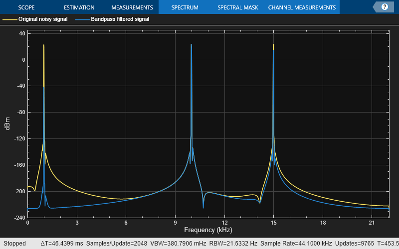
Bandpass filter a discrete-time sine wave signal which consists of three sinusoids at frequencies, 1 kHz, 10 kHz, and 15 kHz.

Design an FIR Equiripple bandpass filter by first creating a bandpass filter design specifications object, and then designing a filter using these specifications.

Design Bandpass Filter

Create a bandpass filter design specifications object using fdesign.bandpass.

bandpassSpecs = fdesign.bandpass('Fst1,Fp1,Fp2,Fst2,Ast1,Ap,Ast2', ...
    1/4,3/8,5/8,6/8,60,1,60);

List the available design methods for this object.

designmethods(bandpassSpecs)

Design Methods for class fdesign.bandpass (Fst1,Fp1,Fp2,Fst2,Ast1,Ap,Ast2):


butter
cheby1
cheby2
ellip
equiripple
kaiserwin

To design an Equiripple filter, pick 'equiripple'.

bpFilter = design(bandpassSpecs,'equiripple',Systemobject=true)

bpFilter = 
  dsp.FIRFilter with properties:

            Structure: 'Direct form'
      NumeratorSource: 'Property'
            Numerator: [-0.0043 -3.0812e-15 0.0136 3.7820e-15 -0.0180 -4.2321e-15 7.1634e-04 4.0993e-15 0.0373 -4.1057e-15 -0.0579 3.7505e-15 0.0078 -3.4246e-15 0.1244 2.4753e-15 -0.2737 -8.6287e-16 0.3396 -8.6287e-16 -0.2737 ... ] (1x37 double)
    InitialConditions: 0

  Use get to show all properties

Visualize the frequency response of the designed filter.

freqz(bpFilter,[],44100)

Figure contains 2 axes objects. Axes object 1 with title Phase, xlabel Frequency (kHz), ylabel Phase (degrees) contains an object of type line. Axes object 2 with title Magnitude, xlabel Frequency (kHz), ylabel Magnitude (dB) contains an object of type line.

Create Sinusoidal Signal

Create a signal that is a sum of three sinusoids with frequencies at 1 kHz, 10 kHz, and 15 kHz. Initialize spectrum analyzer to view the original signal and the filtered signal.

Sine1 = dsp.SineWave(Frequency=1e3,SampleRate=44.1e3,SamplesPerFrame=4000);
Sine2 = dsp.SineWave(Frequency=10e3,SampleRate=44.1e3,SamplesPerFrame=4000);
Sine3 = dsp.SineWave(Frequency=15e3,SampleRate=44.1e3,SamplesPerFrame=4000);

SpecAna = spectrumAnalyzer(PlotAsTwoSidedSpectrum=false, ...
    SampleRate=Sine1.SampleRate, ...
    ShowLegend=true, ...
    YLimits=[-240,45]);

SpecAna.ChannelNames = {'Original noisy signal','Bandpass filtered signal'};

Filter Sinusoidal Signal

Filter the sinusoidal signal using the bandpass filter that has been designed. View the original signal and the filtered signal in the spectrum analyzer. The tone at 1 kHz is filtered out and attenuated. The tone at 10 kHz is unaffected, and the tone at 15 kHz is mildly attenuated because it appears in the transition band of the filter.

for i = 1:5000
    x = Sine1()+Sine2()+Sine3();
    y = bpFilter(x);
    SpecAna(x,y);
end
release(SpecAna)

More About

expand all

Sinusoid

A real-valued, discrete-time sinusoid is defined as:

$y (n) = A \sin (2 π f n + ϕ)$

where A is the amplitude, f is the frequency in Hz, and φ is the initial phase, or phase offset, in radians.

A complex sinusoid is defined as:

$y (n) = A e^{j (2 π f n + ϕ)}$

Algorithms

expand all

Trigonometric Function

The trigonometric function method computes the sinusoid in the ith channel, y_i, by sampling the continuous function

$\begin{array}{l} y_{i} = A_{i} \sin (2 π f_{i} t + ϕ_{i}) & (real) \\ \begin{array}{l} or \end{array} \\ y_{i} = A_{i} e^{j (2 π f_{i} t + ϕ_{i})} & (complex) \end{array}$

with a period of T_s, where you specify T_s in the sample time.

At each sample time, the algorithm evaluates the sine function at the appropriate time value within the first cycle of the sinusoid. By constraining trigonometric evaluations to the first cycle of each sinusoid, the algorithm avoids the imprecision of computing the sine of very large numbers. This constraint also eliminates the possibility of discontinuity during extended operations, when an absolute time variable might overflow. This method therefore avoids the memory demands of the table lookup method at the expense of many more floating-point operations.

Table Lookup

The table lookup method precomputes the unique samples of every output sinusoid at the start of the simulation, and recalls the samples from memory as needed. Because a table of finite length can only be constructed when all output sequences repeat, the method requires that the period of every sinusoid in the output be evenly divisible by the sample period. That is, 1/(f_iT_s) = k_i must be an integer value for every channel i = 1, 2, ..., N.

When the algorithm optimizes the table of sine values for Speed, the table constructed for each channel contains k_i elements. When the optimization is for Memory, the table constructed for each channel contains k_i/4 elements.

For long output sequences, the table lookup method requires far fewer floating-point operations than any of the other methods. However, the method can demand considerably more memory, especially for high sample rates (long tables). This method is recommended for models that are intended to emulate or generate code for DSP hardware, which need to be optimized for execution speed.

Note

The lookup table for this object is constructed from double-precision floating-point values. When you use the Table Lookup computation mode, the maximum amount of precision you can achieve in your output is 53 bits. Setting the word length of the output data type to values greater than 53 bits does not improve the precision of your output.

Differential

The differential method uses an incremental algorithm. This algorithm computes the output samples based on the output values computed at the previous sample time (and precomputed update terms) by making use of the following identities.

$\begin{array}{l} \sin (t + T_{s}) = \sin (t) \cos (T_{s}) + \cos (t) \sin (T_{s}) \\ \cos (t + T_{s}) = \cos (t) \cos (T_{s}) - \sin (t) \sin (T_{s}) \end{array}$

The update equations for the sinusoid in the ith channel, y_i, can therefore be written in matrix form as

$[\begin{matrix} \sin {2 π f_{i} (t + T_{s}) + ϕ_{i}} \\ \cos {2 π f_{i} (t + T_{s}) + ϕ_{i}} \end{matrix}] = [\begin{matrix} \cos (2 π f_{i} T_{s}) & \sin (2 π f_{i} T_{s}) \\ - \sin (2 π f_{i} T_{s}) & \cos (2 π f_{i} T_{s}) \end{matrix}] [\begin{matrix} \sin (2 π f_{i} t + ϕ_{i}) \\ \cos (2 π f_{i} t + ϕ_{i}) \end{matrix}]$

where you specify T_s in the sample time. Since T_s is constant, the right-hand matrix is a constant and can be computed once at the start of the simulation. The value of A_isin[2πf_i(t+T_s)+ϕ_i] is then computed from the values of sin(2πf_it+ϕ_i) and cos(2πf_it+ϕ_i) by a simple matrix multiplication at each time step.

This mode offers reduced computational load, but is subject to drift over time due to cumulative quantization error. Because the method is not contingent on an absolute time value, there is no danger of discontinuity during extended operations, when an absolute time variable might overflow.

Extended Capabilities

C/C++ Code Generation
Generate C and C++ code using MATLAB® Coder™.

Usage notes and limitations:

This object has no tunable properties for code generation.
See System Objects in MATLAB Code Generation (MATLAB Coder).

Version History

Introduced in R2012a

dsp.SineWave

Description

Creation

Syntax

Description

Properties

Amplitude — Amplitude of sine wave 1 (default) | scalar | vector

Dependencies

Frequency — Frequency of sine wave 100 (default) | scalar | vector

PhaseOffset — Phase offset of sine wave 0 (default) | scalar | vector

ComplexOutput — Flag that indicates whether waveform is real or complex false (default) | true

Method — Method used to generate sinusoids 'Trigonometric function' (default) | 'Table lookup' | 'Differential'

TableOptimization — Optimize table of sine values for speed or memory 'Speed' (default) | 'Memory'

Dependencies

SampleRate — Sample rate of output signal 1000 (default) | positive scalar

SamplesPerFrame — Number of samples per frame 1 (default) | positive integer

OutputDataType — Data type of the sine wave output 'double' (default) | 'single' | 'Custom'

CustomOutputDataType — Output word and fraction lengths numerictype([],16) (default) | numerictype([],32,30)

Dependencies

Usage

Syntax

Description

Output Arguments

sineOut — Sine wave output vector | matrix

Object Functions

Common to All System Objects

Examples

Generate a Sine Wave Signal

Filter Frames of a Noisy Sine Wave Signal in MATLAB

Bandpass Filtering of Sinusoids

More About

Sinusoid

Algorithms

Trigonometric Function

Table Lookup

Differential

Extended Capabilities

C/C++ Code Generation Generate C and C++ code using MATLAB® Coder™.

Version History

See Also

Functions

Objects

Topics

`Amplitude` — Amplitude of sine wave
`1` (default) | scalar | vector

`Frequency` — Frequency of sine wave
`100` (default) | scalar | vector

`PhaseOffset` — Phase offset of sine wave
`0` (default) | scalar | vector

`ComplexOutput` — Flag that indicates whether waveform is real or complex
`false` (default) | `true`

`Method` — Method used to generate sinusoids
`'Trigonometric function'` (default) | `'Table lookup'` | `'Differential'`

`TableOptimization` — Optimize table of sine values for speed or memory
`'Speed'` (default) | `'Memory'`

`SampleRate` — Sample rate of output signal
`1000` (default) | positive scalar

`SamplesPerFrame` — Number of samples per frame
`1` (default) | positive integer

`OutputDataType` — Data type of the sine wave output
`'double'` (default) | `'single'` | `'Custom'`

`CustomOutputDataType` — Output word and fraction lengths
`numerictype([],16)` (default) | `numerictype([],32,30)`

`sineOut` — Sine wave output
vector | matrix

C/C++ Code Generation
Generate C and C++ code using MATLAB® Coder™.