Time Scope Measurements
This example shows how to measure performance characteristics of a pulse width modulated sinusoid. The example contains a model, which you can modify to view the effects of parameter changes on rise time, fall time, overshoot, undershoot, pulse width, pulse period, and duty cycle measurements. The example also models a rising edge trigger and you can perform basic statistical operations (mean, median, RMS, maximum, minimum) and measure the frequency and period of the pulse period via cursors and peak finding.
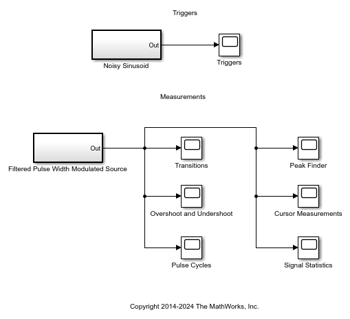
The example model contains several measurements and their corresponding setups. Open the TimeScopeMeasurements example model.

Triggers
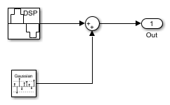
The Noisy Sinusoid block shows how to use a trigger to stabilize a noisy sinusoid in the display. You can see how the sinusoid is constructed by double-clicking the Noisy Sinusoid block.

The sinusoidal signal is fed into a Time Scope block with triggers enabled.


You can experiment with the trigger position by dragging the markers around the display. You can trigger upon rising or falling edges. This example includes 0.1 V of hysteresis to help stabilize the sinusoid in the presence of noise. The hysteresis ensures that the signal traverses at least 0.1 V below the trigger level before registering a positive-going transition.
If you close the triggers, you will see that the sinusoid no longer stays fixed on the screen. You can bring the triggers back by clicking the trigger icon.
Measurements of Pulse-Width Modulated Source
In this example, a pulse-width modulated source is connected to several time scopes that contain measurements.
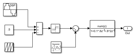
You can view the source by clicking it in the model:

The model constructs sinusoidal pulse-width modulation by applying a bias to the desired sine wave and subsequently subtracting a periodic sawtooth wave. The resulting waveform is then fed to a comparator to form the shape of the pulse. Noise is then added to the signal and the signal is then sent to a filter with an underdamped response.
You can modify the amount of additive noise on the input by clicking the Random Source block and modifying the variance of the Gaussian distribution.
You can similarly modify the response of the filter by changing its coefficients.
Transitions
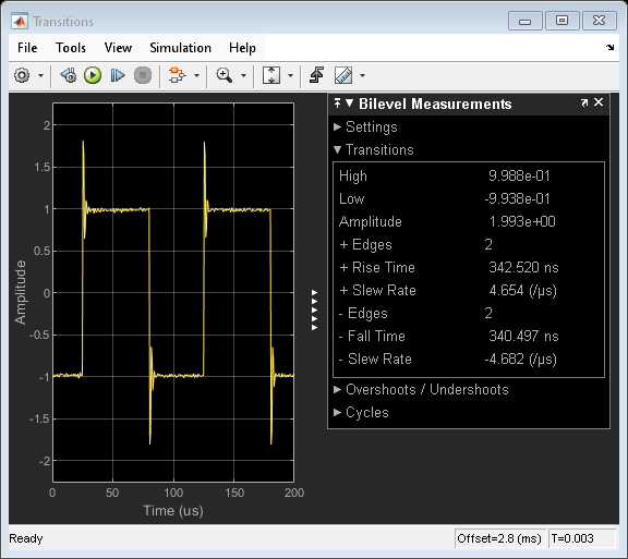
You can view some basic information about the rising and falling transitions of the waveform by viewing the Transitions pane in the Bilevel Measurements dialog box.
Viewing the results, you can see that the pulse has a high voltage level of +1 V and a low voltage level of -1 V.
This image shows two rising (positive) edges and two falling (negative) edges with rise times and fall times of around 340 ns. If you zoom in on just one edge of the waveform you can see the measurements for just that edge.
The edges of the pulses are fairly steep, with a slew rate of about 4 V/us. The example uses an underdampened filter to achieve this rate. Changing to an overdamped filter will decrease the rate at which the edge of each pulse can transition between pulse levels. The output of an underdampened filter exhibits significant ringing immediately after changing between low and high states. To quantify this ringing behavior, you can use the measurements in the Overshoots / Undershoots list.
Overshoot and Undershoot
The Bilevel Measurements dialog box also contains measurements that relate to an underdampened environment. You can view the transition aberrations by opening the Overshoots / Undershoots list.
The average overshoot of the rising edges is about 42%. The undershoot is 34%. Large overshoots can sometimes damage logic devices that are designed to accept only a small voltage range. Large undershoots can cause devices to detect incorrect logic states. In this example, the transitions settle on an average within 7.3 microseconds.
You can reduce the amount of ringing by experimenting with the filter coefficients at the output of the modulated source.
Pulse Cycles
You can also view how the pulse width and duty cycle vary as functions of time by expanding the Cycles list in the Bilevel Measurements dialog box.
This example shows three positive-polarity pulses but only two negative-polarity pulses. The pulse frequency is 10 kHz. You can observe the encoded sinusoid by watching how the duty cycle and pulse width change over time.
Peak Finder
Alternatively, you can measure the amplitudes and the times of significant peaks from the Peak Finder dialog box.
The voltage at the tip of each overshoot is about 1.8 V and the next largest ringing component of the first pulse is at 1.14 V.
Expand the settings panel to change the number of peaks shown. You can also filter based on height or distance between peaks. You can also change the text annotation shown in the display.
Cursor Measurements
You can measure the relative distances between events of the waveform by using cursor measurements. Here the cursors are at the start of each pulse and confirm that the pulse period is 10 kHz.
Experiment with the settings to move the cursors anywhere on the screen or measure the locations of other signals. You can move the cursors with the arrow keys and also snap them to either the nearest data point or screen pixel.
Signal Statistics
You can view basic signal statistics of the captured wave with the Signals Statistics measurement dialog box.
You can observe the minimum and maximum values of the displayed signal and other signal metrics, such as the peak-to-peak, mean, median, and RMS values.
References
IEEE Std. 181-2003 IEEE Standard on Transitions, Pulse, and Related Waveforms