DSP HDL IP Designer
Configure and generate HDL code for digital signal processing IP cores
Since R2024b
Description
Use the DSP HDL IP Designer app to select a digital signal processing (DSP) algorithm and configure parameters and input stimulus. Then, generate HDL code and a testbench to verify the behavior of your design.
The app enables you to select and configure hardware-optimized algorithms and generate HDL code for those algorithms. The app provides algorithms that have streaming data interfaces and hardware-friendly control signals. The algorithms can use frame-based input and parallel operations to achieve gigasamples-per-second (GSPS) data rates, also called super sample rates. You can change the algorithm parameters to explore and generate different hardware implementations. The app supports HDL code generation and optional generation of an HDL testbench. To generate HDL code and testbench you must have the HDL Coder™ product. If you have the HDL Verifier™ product, you can generate a cosimulation testbench or a DPI component for your algorithm.
To get started, see Generate and Verify HDL Code with DSP HDL IP Designer App.
You can save and restore your IP design session by using the buttons on the toolbar. When you save a session, the app creates a
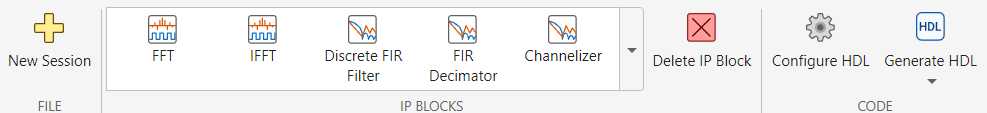
.matfile with the name you specify. (since R2025a)You can configure and generate HDL code for one algorithm at a time. Select your algorithm from the IP Blocks gallery.
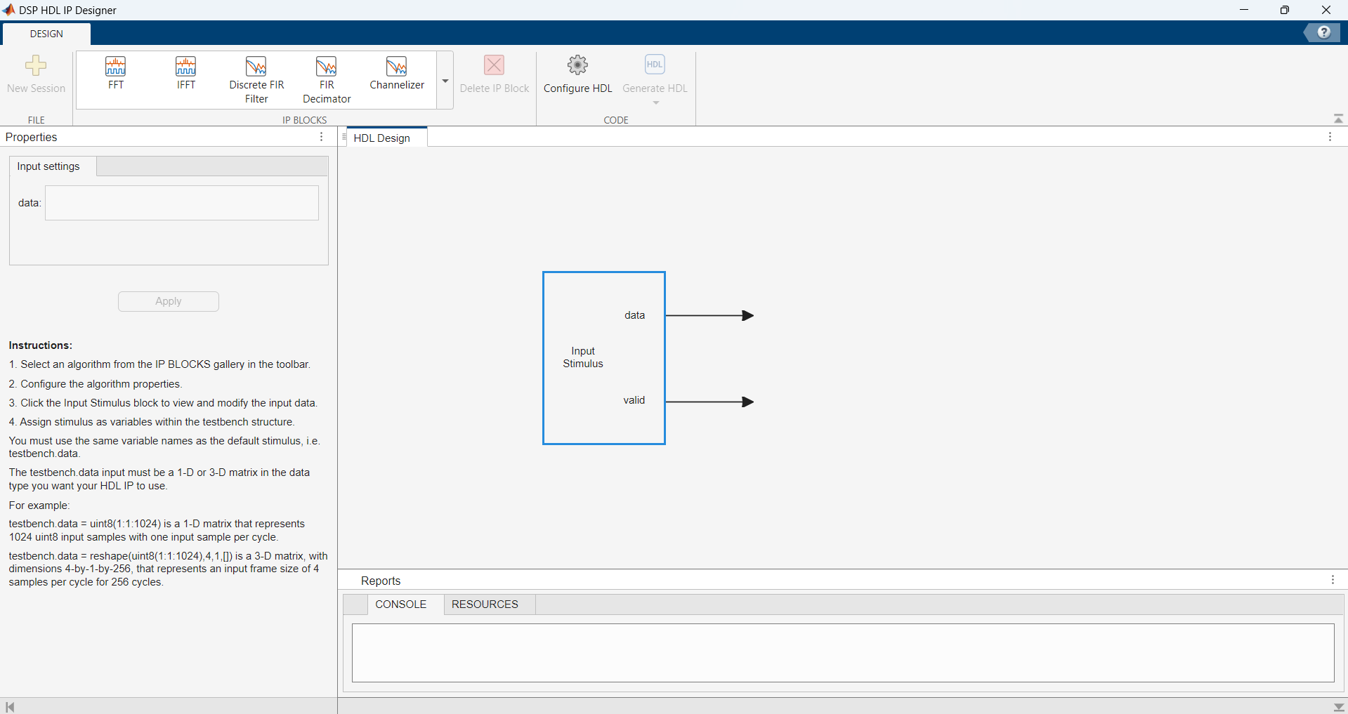
Click the Input Stimulus block to configure input data signals. The dimensions and data types of these values define your HDL interface, and the generated testbench applies these values to your algorithm. You do not have to specify stimulus for input control signals. The app provides default values for each input port, assigned as fields in the
testbenchstructure. For help creating input stimulus, see Setting Input Stimulus.When you design biquad or discrete FIR filters, you can use the Analyze button in the toolbar to open the Filter Analyzer app and visualize the characteristics of the filter. (since R2025a)
To configure HDL code generation options, including enabling generation of an HDL simulator testbench, click Configure HDL. For more information about the available options, see Parameters. Then, to generate code, click Generate HDL. After you generate HDL code, you can see output log messages on the Console tab and a hardware resources estimate on the Resources tab. You must have the HDL Coder product to generate HDL code.
To generate a cosimulation testbench, set options in the EDA Scripts and Cosimulation tab of the Configure HDL menu. For more information about the available options, see EDA Scripts and Cosimulation. You must have the HDL Verifier product to use the cosimulation testbench feature.
To generate a SystemVerilog DPI component, select Generate DPI Component from the Generate HDL menu. You can integrate this component into your HDL simulation as a behavioral model. You must have the HDL Verifier product to use the Generate DPI Component feature.
You can export your designs as either a MATLAB® script file or a Simulink® model that includes your configured algorithm and input stimulus, and simulates your algorithm. For more details see Export Algorithm to MATLAB and Export Algorithm to Simulink. (since R2025a)
Open the DSP HDL IP Designer App
MATLAB Toolstrip: On the Apps tab, under Signal Processing and Audio, click the app icon.
MATLAB command prompt: Enter
dsphdlIPDesigner.MATLAB command prompt: Load a preconfigured System object™ into the app by entering
dsphdlIPDesigner(ObjVariable). For which objects are supported, see Generate HDL for Preconfigured Algorithm with DSP HDL IP Designer App. (since R2025a)Filter Designer (Signal Processing Toolbox) app: Under the Export menu, select Export to DSP HDL IP Designer. For which filters are supported, see Generate HDL for Preconfigured Algorithm with DSP HDL IP Designer App. (since R2026a)
Examples
This example shows how to configure a discrete FIR filter and generate HDL code in the DSP HDL IP Designer app.
To generate HDL IP core for an algorithm in the DSP HDL IP Designer app:
Select an algorithm and set its parameters.
Configure input dimensions and data types.
Generate HDL code and, optionally, testbenches.
This example shows designs for a fully parallel FIR filter with high throughput and a partly serial FIR filter that uses fewer resources and has lower throughput. For details of filter implementation options, see FIR Filter Architectures for FPGAs and ASICs.
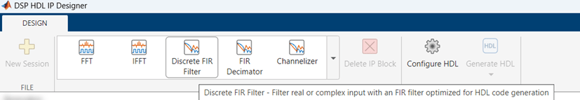
Each IP block in the app provides the same implementation, ports, and parameters as the Simulink® library block for the same algorithm. For more information about the ports and parameters of each algorithm, see the block reference pages. For example, see Discrete FIR Filter.
Open the App
In the apps gallery, under the Signal Processing and Audio group, click the DSP HDL IP Designer app. Alternatively, at the MATLAB® command prompt, enter dsphdlIPDesigner.
Select Algorithm
Select the Discrete FIR Filter from the IP Blocks gallery in the app.
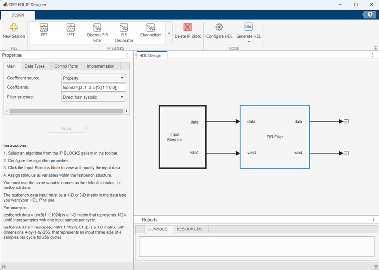
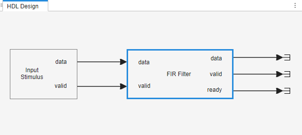
All the algorithms have streaming interfaces with a data port and a control signal that indicates when the input data is valid. The data ports accept and return a scalar or small vector of input data samples on each clock cycle. In the app, you can see the interface signals connecting the IP block to the Input Stimulus block.
To configure your algorithms, set options in the Properties sidebar. Setting the Filter Structure parameter to Direct-form systolic implements a fully parallel filter with high throughput. Configure the filter coefficients as a 25-tap lowpass FIR filter by setting the Coefficients parameter to firpm(24,[0 .1 .3 .5]*2,[1 1 0 0]). The coefficients are specified as double data type and, by default, the filter casts them to match the input data type. You can also specify a coefficient data type on the Data Types tab. The IP block displays the latency of the algorithm, from first input to first output, assuming input data is valid every cycle. For this filter implementation, the latency is 20 cycles.
Configure Input Stimulus
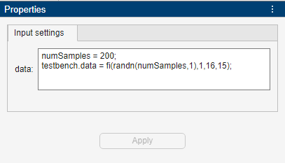
Click the Input Stimulus block. The Input settings section in the Properties sidebar provides dimensions and data types for the input to the algorithm. The app provides default values for each input port. The dimensions and data types of these values define your HDL interface, and the generated testbench applies these values to your algorithm. You do not need to specify values for control signals like valid and reset. The generated testbench automatically drives the control signals. For this algorithm, you must specify the data input.
The data input for this FIR filter can be a 1-D or 3-D matrix. A 1-D matrix represents a stream of data samples over time. A 3-D matrix represents number of input samples per cycle-by-number of data channels-by-data samples over time. The Discrete FIR Filter algorithm supports frame-based data, or multichannel data, but not both at the same time.
This example specifies a 1-D matrix that represents 200 fixed-point data type input samples. This data format configures the filter to accept one input sample each clock cycle and the filter has a single data channel.
numSamples = 200;
testbench.data = fi(randn(numSamples,1),1,16,15);
Alternatively, to configure the filter to accept a frame of four input samples each clock cycle, you can set the input data to a 4-by-1-by-data samples over time matrix. A filter with frame-based input must have a single data channel. A filter with 4-sample vector input implements a polyphase decomposition into four parallel subfilters and does not implement symmetry optimizations. This implementation uses more resources to support increased throughput. The IP block updates the displayed latency to 16 cycles for this implementation.
numSamples = 200;
dataIn = fi(randn(numSamples,1),1,16,15);
testbench.data = reshape(dataIn,4,1,[]);
To specify a multichannel filter, first set the Coefficients parameter to a number of channels-by-coefficients matrix, like [firpm(24,[0 .1 .3 .5]*2,[1 1 0 0]); firpm(24,[0 .1 .2 .4]*2,[1 1 0 0])]. Then, configure the input stimulus as a 3-D matrix of 1-by-number of channels-by-data samples over time values. A filter with multiple channels cannot use frame-based input. Each channel accepts a single sample each cycle. This filter uses the same resources as the scalar input filter and displays a latency of 21 cycles.
numSamples = 200;
dataIn = fi(randn(numSamples,1),1,16,15);
testbench.data = reshape(dataIn,1,2,[]);
Generate HDL Code
You can configure HDL code generation options in Configure HDL. By default, the app generates an HDL simulator testbench and scripts for compiling and running the design in the Siemens® ModelSim® and AMD® Vivado® simulators. The HDL simulator testbench applies the input signals you defined in Input Stimulus, drives the input control signals, and compares all the output ports of the generated HDL IP block against the output from running your algorithm in a MATLAB® simulation.
To generate HDL code and a testbench, click Generate HDL. The code generation log appears in the Console window, including any warning or error messages. These results are for the scalar-input, single channel, fully parallel filter implementation.
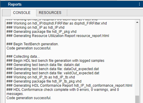
The generated files and reports are under codegen\hdl_IP\hdlsrc in your working folder. You can find more information about any errors or warnings in the hdl_IP_hdl_conformance_report.html file.
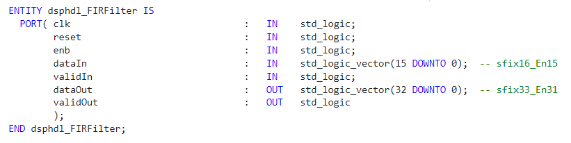
The generated VHDL entity shows the IP block interface, including control signals and the input data type that you specified. The output data type is determined by the Output parameter on the Data Type tab of the algorithm. By default, it is derived from the input data type with no loss of precision.
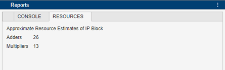
The Resources tab shows an estimate of hardware resources used by this filter implementation. A filter with scalar input shares multipliers between symmetric coefficients, so this 25-tap filter uses 13 multipliers.
Serial Filter Implementation
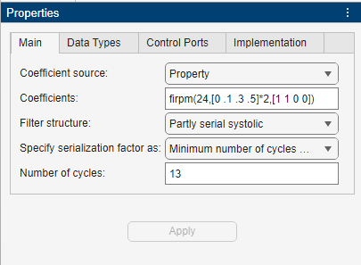
To implement a filter that uses fewer resources but has lower throughput, you can select a serial implementation. On the FIR Filter block in the app, set the Structure parameter to Partly serial systolic. Then, you can specify the serialization by either the number of multipliers or number of cycles between valid input samples. For a filter with L coefficients, the IP block implements a serial filter with M or fewer multipliers and requires input samples that are at least N cycles apart, such that L = N × M. To implement a fully serial filter, select Minimum number of cycles between valid input samples and set Number of cycles to 13 (the number of unique coefficients, and the number of multipliers used by the scalar input fully parallel filter).
When you apply these changes, the IP block in the app now has an output ready port that indicates when the filter is ready for new input data. The generated HDL testbench automatically responds to the ready signal and spaces the input data samples the correct number of cycles apart. You can use the same Input Stimulus as the fully-parallel implementation. The app displays a latency of 20 cycles on the IP block. The latency for a fully serial implementation of a symmetric single channel filter is L + 7 cycles. For the serial implementation, the latency represents the cycles from first input to first output, and it does not depend on the input valid after the first data.
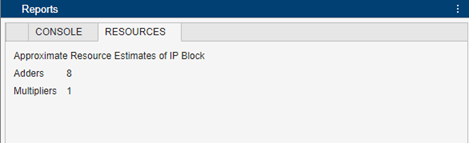
After you generate HDL code, you can see the updated resource estimate on the Resources tab. This implementation uses only one multiplier but has slower throughput than the parallel filter because samples can be applied only every 13 cycles. The single multiplier is shared in time between the symmetry-optimized coefficients.
Using the app you can explore hardware implementations of algorithms without constructing a model or script to run the algorithm. You can quickly generate HDL code and testbench components for your algorithms, and assess the hardware resource use of your IP block.
This example shows how to configure a programmable CIC Decimator algorithm in the DSP HDL IP Designer app, and then export the design and input stimulus as MATLAB® scripts.
This example includes a MAT file that loads the algorithm and HDL code generation settings into the app. It also includes the exported MATLAB script files.
Open the DSP HDL IP Designer app and click Open Session. Load the app-cicdecim-ex.mat file. The file configures a CIC Decimator algorithm with the Decimation factor source parameter set to Input port and the largest expected decimation factor, Decimation factor (Rmax) parameter, set to 12. In this configuration, the algorithm has an input port R for the decimation factor, and accepts and returns scalar data samples. The IP block usually displays its latency, but in this case the latency depends on the input R value, so the block does not display a latency.

Click the Input Stimulus block to see the default values for the input. The input decimation factor must be data type fixdt(0,12,0) and must be an integer in the range from 1 to the Decimation factor (Rmax) value. In the input stimulus code, the testbench.R value must be a scalar. This value represents the dimension and data type of the input. The testbench.data value represents the dimensions and data type of the input samples, and specifies how many samples to apply over time in the testbench.

In the toolbar, click Export > Export to MATLAB. The app saves files named export_DesignName.m and export_DesignName_tb.m. DesignName is the value of the Name parameter in the Configure HDL menu.
The export_progCICDecim.m file contains a dsphdl.CICDecimator System object™ configured with the same settings as the algorithm in the app.
function [dataOut,validOut] = export_progCICDecim(dataIn,validIn,RIn)
% Generated by HDL IP Designer.

persistent ipblock

if isempty(ipblock)
    ipblock = dsphdl.CICDecimator( ...
        'DecimationSource','Input port', ...
        'MaxDecimationFactor',12, ...
        'GainCorrection',true);
end

[dataOut,validOut] = ipblock(dataIn,validIn,RIn);

end
The export_progCICDecim_tb.m file contains code that assigns the stimulus values from the Input Stimulus block in the app, and code that calls the System object to simulate the algorithm. You can modify the _tb file to apply other input values, and analyze the output data.
%Testbench generated using HDL IP Designer
%
% generate input stimulus for DUT
fs = 44.1e3; % Original sampling frequency: 44.1 kHz
n = (0:1023); % 1024 samples
x = fi(sin(2*pi*1e3/fs*n),true,16,8);
testbench.data = reshape(x,size(x,2),size(x,1));
data = testbench.data ;

% R value must be scalar
testbench.R = fi(2,0,12,0);
R = testbench.R ;
R = repmat(testbench.R,1024,1);

NumDim = length(size(data));
NumSamples = size(data,1);
SamplesPerFrame = 1;
NumChannels = size(data,2);

valid = true(1,NumSamples);
dataIn = data;
validIn = valid;
RIn = R;

% call DUT with stimulus and save output
for ii = 1:1:NumSamples
   [dataOut(ii), validOut(ii)] = export_progCICDecim(dataIn(ii), validIn(ii), RIn(ii));
end
For instance, in export_progCICDecim_tbEx.m, this example sets the R input to change every 265 input samples.
  testbench.R = fi([2,4,8,2],0,12,0);
  R = [repmat(testbench.R(1),256,1);repmat(testbench.R(2),256,1);repmat(testbench.R(3),256,1);repmat(testbench.R(4),256,1)];
Run export_progCICDecim_tbEx.m and display the results of simulating the System object with the new R values by using the dsp.LogicAnalyzer object. In the waveform, you can see the changing R value and the effect on the output valid pattern after decimation.
export_progCICDecim_tbEx
analyzer = dsp.LogicAnalyzer( ...
    'Name', 'CIC Decim Waveform', ...
    'NumInputPorts', 5, ...
    'DisplayChannelRadix', 'Hexadecimal', ...
    'SampleTime', 1, ...
    'TimeSpan',1024);
modifyDisplayChannel(analyzer, 1, 'Name', 'dataIn');
modifyDisplayChannel(analyzer, 2, 'Name', 'validIn');
modifyDisplayChannel(analyzer, 3, 'Name', 'R');
modifyDisplayChannel(analyzer, 4, 'Name', 'dataOut');
modifyDisplayChannel(analyzer, 5, 'Name', 'validOut');
analyzer(dataIn, validIn', RIn, dataOut', validOut');

This example shows how to configure a programmable CIC Interpolator algorithm in the DSP HDL IP Designer app, and export the design and input stimulus as a Simulink® model.
This example includes a MAT file that loads the algorithm and HDL code generation settings into the app. It also includes the exported Simulink model file.
Open the DSP HDL IP Designer app and click Open Session. Load the app-cicinterp-ex.mat file. The file configures a CIC Interpolator algorithm with the Interpolator factor source parameter set to Input port and the largest expected interpolation factor, Interpolation factor (Rmax) parameter, set to 12. In this configuration, the algorithm has an input port R for the interpolation factor, and accepts and returns scalar data samples. Because interpolation requires more output cycles than input cycles, the algorithm also has a backpressure signal, ready, that indicates when the algorithm is ready to accept new input samples. The IP block usually displays its latency, but in this case, the latency depends on the input R value, so no latency is displayed.

Click the Input Stimulus block to see the default values for the input. The input interpolation factor must be data type fixdt(0,12,0) and must be an integer in the range from 1 to the Interpolation factor (Rmax) value. In Input Stimulus, the testbench.R value must be a scalar. This value represents the dimension and data type of the input. The testbench.data value represents the dimensions and data type of the input samples, and specifies how many samples to apply over time in the testbench.

In the toolbar, click Export > Export to Simulink. The app opens a Simulink model that contains a CIC Interpolator block configured with the same settings as the algorithm in the app.
open_system(export_progCICInterp)

The InitFcn callback of the model assigns the input stimulus to workspace variables, and creates values for input control signals. To view and edit the InitFcn callback, from the Model Settings drop-down menu, open Model Properties and select the Callbacks tab.
%Testbench generated using HDL IP Designer
% generate input stimulus for DUT
fs = 22.05e3; % Original sampling frequency: 22.05 kHz
n = (0:511); % 512 samples
x = fi(sin(2*pi*1e3/fs*n),true,16,8)';
testbench.data = x;
data = testbench.data ;
% R value must be scalar
testbench.R = fi(2,0,12,0);
R = testbench.R ;
R = repmat(testbench.R,512,1);
NumDim = length(size(data));
NumSamples = size(data,1);
SamplesPerFrame = 1;
NumChannels = size(data,2);
valid = true(1,NumSamples);
dataIn = data;
validIn = valid;
RIn = R;
simTime = NumSamples+100;
The exported model is configured to capture the input and output signals of your algorithm to the Logic Analyzer waveform viewer. You can modify the model to apply other input values, or analyze the output data.
For instance, in export_progCICDecim.slx, this example sets the input interpolation factor, R, to a different value every 128 input samples. Because the backpressure signal slows the input rate for larger interpolation factors, the example modifies the simTime setting of the model to allow time to apply all 512 input samples.
testbench.R = fi([2,4,8,2],0,12,0);
R = [repmat(testbench.R(1),256,1);repmat(testbench.R(2),256,1);repmat(testbench.R(3),256,1);repmat(testbench.R(4),256,1)];
...
simTime = NumSamples*4;
Run export_progCICInterp.slx and observe the results of simulating the block with the new R values in the Logic Analyzer. You can see the changing R value and the effect on the backpressure signal and output valid pattern after interpolation.

Related Examples
Parameters
Setting Input Stimulus
After you select your algorithm and set its parameters, click the Input
Stimulus block to configure input data signals. The dimensions and data types of
these values define your HDL interface, and the generated testbench applies these values to
your algorithm. You do not have to specify stimulus for input control signals. The app
provides default values for each input port, assigned as fields in the
testbench structure. You must use the same field names as the default
stimulus.
The testbench.data input must be a 1-D or 3-D matrix in the data type
that you want your HDL IP core to use. A 1-D matrix represents a stream of data samples over
time. A 3-D matrix represents number of input samples per
cycle-by-number of data channels-by-data samples
over time. For example:
testbench.data = uint8(1:1:1024)is a 1-D matrix that represents 1024uint8input samples with one input sample per cycle.testbench.data = reshape(uint8(1:1:1024),4,1,[])is a 3-D matrix, with dimensions 4-by-1-by-256, that represents an input frame size of 4 samples per cycle for 256 cycles.testbench.data = reshape(uint8(1:1:1024),1,2,[])is a 3-D matrix, with dimensions 1-by-2-by-512, that represents 2 channels, each with one input sample per cycle, for 512 cycles. Multichannel filters do not support frame-based input.
Other input signals can be scalars or vectors. For example:
testbench.coeff = fi(fir1(17,0.1),1,16)is a single set of filter coefficients, specified as a 1-by-18 vector of 16-bit fixed-point values.testbench.R = fi(2,0,12,0)is a decimation factor input, specified as a scalar 12-bit integer value.
Some algorithms have a dependency between the algorithm properties and the ports and dimensions of the input stimulus. Configure the properties and input stimulus to match before clicking Apply. The Apply action incorporates any changes from properties and from input stimulus.
You can enter code that generates your input values. Because this code is also used in HDL code generation, it must follow the same limitations as in the testbench file specified for MATLAB to HDL code generation. See Using Test Benches With HDL and HLS Code Generation (HDL Coder).
The input stimulus code cannot directly access workspace variables. To make use of
existing workspace data, call
evalin('base',<expression>).