Generate Generic C/C++ for Sequence-to-Sequence Deep Learning Simulink Models

Prerequisites

For PIL verification, you will need:

Pretrained RUL Network

This example uses a pretrained LSTM network to predict the remaining useful life of an engine, measured in cycles. The LSTM network consists of an LSTM layer with 200 hidden units, followed by a fully connected layer of size 50 and a dropout layer with dropout probability 0.5.The network was trained using the Turbofan Engine Degradation Simulation Data Set as described in [1]. The training data contains simulated time series data for 100 engines. Each sequence varies in length and corresponds to a full run to failure (RTF) instance. The test data contains 100 partial sequences and corresponding values of the remaining useful life at the end of each sequence. For more information on training the network, see the example Sequence-to-Sequence Regression Using Deep Learning (Deep Learning Toolbox).

net = coder.loadDeepLearningNetwork('rulNetwork.mat')

net = 
  SeriesNetwork with properties:

         Layers: [6×1 nnet.cnn.layer.Layer]
     InputNames: {'sequenceinput'}
    OutputNames: {'regressionoutput'}

For information on the networks, layers, and classes supported for code generation, see Networks and Layers Supported for Code Generation.

Download and Prepare Test Data

This section summarizes the steps to download and prepare the test data that this example uses. For more information on the Turbofan Engine Degradation Simulation data set and the preprocessing steps, see the example Sequence-to-Sequence Regression Using Deep Learning (Deep Learning Toolbox).

Download Data Set

Create a directory to store the Turbofan Engine Degradation Simulation data set.

dataFolder = fullfile(tempdir,"turbofan");
if ~exist(dataFolder,'dir')
    mkdir(dataFolder);
end

Download and extract the Turbofan Engine Degradation Simulation data set.

filename = matlab.internal.examples.downloadSupportFile("nnet","data/TurbofanEngineDegradationSimulationData.zip");
unzip(filename,dataFolder)

Calculate Mean and Standard Deviation of Training Data

In the following step, you normalize the test predictors using the mean and standard deviation of the training data. So, you must first use the training data to calculate these normalization parameters.

Load the training data, each column is one observation, each row is one feature. Remove the features that have constant values.

filenamePredictors = fullfile(dataFolder,"train_FD001.txt");
[XTrain] = processTurboFanDataTrain(filenamePredictors);

m = min([XTrain{:}],[],2);
M = max([XTrain{:}],[],2);
idxConstant = M == m;

for i = 1:numel(XTrain)
    XTrain{i}(idxConstant,:) = [];
end

Calculate the mean and standard deviation over all observations.

mu = mean([XTrain{:}],2);
sig = std([XTrain{:}],0,2);

Prepare Test Data

Prepare the test data using the function processTurboFanDataTest attached to this example. The function processTurboFanDataTest extracts the data from filenamePredictors and filenameResponses and returns the cell arrays XValidate and YValidate, which contain the test predictor and response sequences, respectively.

filenamePredictors = fullfile(dataFolder,"test_FD001.txt");
filenameResponses = fullfile(dataFolder,"RUL_FD001.txt");
[XValidate,YValidate] = processTurboFanDataTest(filenamePredictors,filenameResponses);

Remove features with constant values using idxConstant calculated from the training data. Normalize the test predictors using the parameters mu and sig calculated from the training data. Clip the test responses at the threshold 150. This same clipping threshold was used on the training data while training the network.

thr = 150;
for i = 1:numel(XValidate)
    XValidate{i}(idxConstant,:) = [];
    XValidate{i} = (XValidate{i} -  mu) ./ sig;
    YValidate{i}(YValidate{i} > thr) = thr;
end

To make the input validation data compatible with Simulink code generation, the sequence lengths for each of the independent 100 observations are zero-padded to create uniformly-sized, 17-by-303 input arrays.

sequenceLengths = cellfun(@length,XValidate,'UniformOutput',true);
maxSequenceLen = max(sequenceLengths);
padFcn = @(x) [x,zeros(size(x,1),maxSequenceLen-size(x,2))];             
XValidatePad = cellfun(padFcn,XValidate,'UniformOutput',false);

The padded values are then converted to a 17-by-303-100 numeric array. To import this data into the Simulink model, specify a structure variable containing the data values and an empty time vector. During simulation, the input for the first time step is read from the first 17-by-303 element of the array. The value for the second time step is read from the second element, and so on, for a total of 100 steps.

simin.time = [];
simin.signals.values = cell2mat(reshape(XValidatePad,1,1,[]));
simin.signals.dimensions = size(XValidatePad{1});

Simulink Model for Prediction

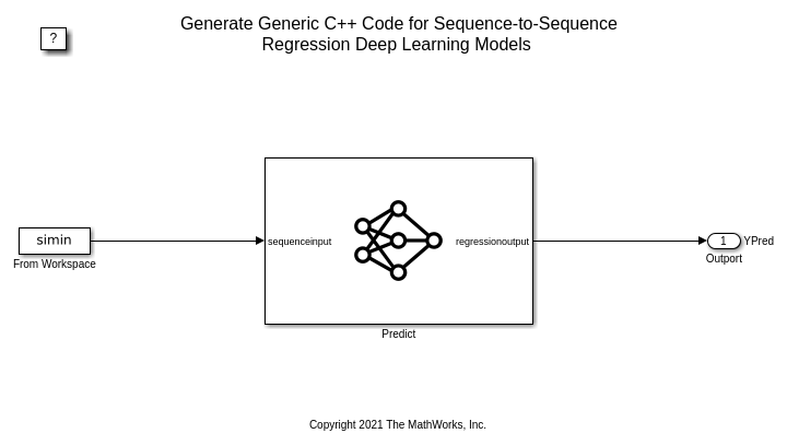
The Simulink model for predicting the remaining useful life of a turbofan engine is shown. The model uses the Predict block from the Deep Neural Networks library that imports the trained network from a rulNetwork MAT-file. Additionally, the Mini-batch size parameter of the block is set to 1.

model = 'rulPredict';
open_system(model)

Run the Simulation

To validate the Simulink model, run the simulation.

set_param(model,'SimulationMode','Normal');
sim(model);

The output YPred of the Simulink model contains the predicted remaining useful life values from the network. This output is first trimmed to remove the results from the zero-padded values and then converted to a cell array.

YPred_cell = squeeze(mat2cell(YPred,1,maxSequenceLen,ones(1,100)));

for t = 1:length(sequenceLengths)   
    YPred_cell{t}(:,sequenceLengths(t) + 1:end) = [];
end 

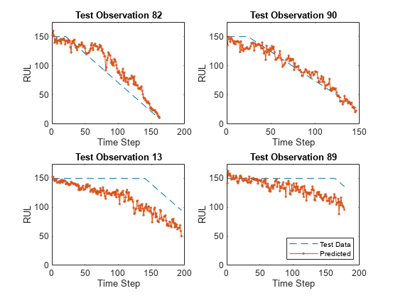
Plot the predicted remaining useful life (RUL) values for four randomly-selected observations and compare them to the validation data.

observationIdx = randperm(100,4);
rulExamplePlots(observationIdx,YValidate,YPred_cell);

Configure Model for Code Generation

To generate C/C++ code that does not depend on any third-party deep learning libraries and build an executable, select the generic real-time (ERT) target from Embedded Coder.

cs = getActiveConfigSet(model);
switchTarget(cs,'ert.tlc',[]);

Configure code generation specific parameters. Setting MAT-file logging enables the generated code to redirect simulation data to a MAT-file.

set_param(cs,'TargetLang','C');
set_param(cs,'Toolchain','Automatically locate an installed toolchain');
set_param(cs,'ObjectivePriorities','Execution efficiency');
set_param(cs,'DLTargetLibrary','None');
set_param(cs,'GenerateReport','on');
set_param(cs,'CodeInterfacePackaging','Nonreusable function'); 
set_param(cs,'MatFileLogging', 'on');

Generate and Build the Simulink Model

Generate and build the Simulink model by using the slbuild command. The code generator places the files in a build folder, a subfolder named rulPredict_ert_rtw under your current working folder.

evalc("slbuild('rulPredict')");

Run the Generated Executable

Run the generated executable. After successful execution, the rulPredict executable creates a rulPredict MAT-file in the current working folder.

if ispc
    status = system('rulPredict.exe');
else
    status = system('./rulPredict');
end 

** created rulPredict.mat ** 
 

load('rulPredict.mat')

The output rt_YPred contains the predicted remaining useful life values from the network. This output is first trimmed to remove the results from the zero-padded values and then converted to a cell array.

rt_YPred_cell = squeeze(mat2cell(rt_YPred,1,maxSequenceLen,ones(1,100)));

for t = 1:length(sequenceLengths)   
    rt_YPred_cell{t}(:,sequenceLengths(t) + 1:end) = [];
end 

Plot the predicted remaining useful life (RUL) values for four randomly-selected observations and compare them to the validation data.

rulExamplePlots(observationIdx,YValidate,rt_YPred_cell);

Code Verification with Processor-in-the-Loop (PIL) Simulation

To ensure that the behavior of the deployment code matches the design, you can configure the Simulink model to run a PIL simulation on embedded boards. In a PIL simulation, the generated code runs on embedded boards such as the STMicroelectronics® Discovery. The results of the PIL simulation are transferred to Simulink to verify numerical equivalence of the simulation and the code generation results.

This example shows PIL verification on the STMicroelectronics Discovery board by using the Embedded Coder® Support Package for STMicroelectronics Discovery Boards. This example is pre-configured to run on the STM32F746G-Discovery board. You can configure this model to use other supported embedded boards by selecting them as the "Hardware board" on the Hardware Implementation pane of the Model Configuration Parameters.

Prepare Test Data

For PIL simulation, this example sorts the observations by sequence length and picks the first 10. These observations are zero-padded to create uniformly-sized, 17-by-54 input arrays. The padded values are then converted to a 17-by-54-10 numeric array. To import this data into the Simulink model, specify a structure variable containing the data values and an empty time vector. During simulation, the input for the first time step is read from the first 17-by-54 element of the array. The value for the second time step is read from the second element, and so on, for a total of 10 steps.

[~,idx] = sort(cellfun(@length,XValidate));
XValidatePIL = XValidate(idx(1:10));
YValidatePIL = YValidate(idx(1:10));
sequenceLengths = cellfun(@length,XValidatePIL,'UniformOutput',true);
maxSequenceLen = max(sequenceLengths);
padFcn = @(x) [x,zeros(size(x,1),maxSequenceLen-size(x,2))];             
XValidatePILPad = cellfun(padFcn,XValidatePIL,'UniformOutput',false);
simin.time = [];
simin.signals.values = cell2mat(reshape(XValidatePILPad,1,1,[]));
simin.signals.dimensions = size(XValidatePILPad{1});

Top Model PIL

The rulPredict_pil is a modified version of the rulPredict model for PIL verification. To load the test vectors, the rulPredict_pil model replaces the From Workspace block with an Inport block. The Inport block is configured to accept a 17-by-54 array of double data type.

pilModel = 'rulPredict_pil';
open_system(pilModel);

Configure the rulPredict_pil model for the STM32F467G-Discovery target.

cs = getActiveConfigSet(pilModel);
set_param(cs,'HardwareBoard','STM32F746G-Discovery');
set_param(cs,'Toolchain','GNU Tools for ARM Embedded Processors');

The STM32F4-Discovery board supports two different communication interfaces for PIL: ST-LINK and serial. The ST-LINK communication interface does not require any additional cables or hardware besides a USB type A to Mini-B cable used to connect the STM32F4-Discovery board to the host computer. The serial communication interface requires a USB TTL-232 cable. Running a PIL simulation using the serial communication interface is much faster than the running a PIL simulation using ST-LINK. This example is configured to use the serial interface.

Additionally, you must set the COM port parameter in Configuration Parameters > Hardware Implementation > Target Hardware Resources > PIL to match the port number of the serial interface on your Windows computer.

Run PIL Simulation

To compare the PIL results with simulation, run the rulPredict_pil model in normal mode and then in PIL mode.

set_param(cs,'LoadExternalInput','on');
set_param(cs, 'ExternalInput','simin');
set_param(pilModel,'SimulationMode','Normal');

sim(pilModel);
YPred_ref = YPred_pil;

set_param(pilModel,'SimulationMode','Processor-in-the-Loop (PIL)')
sim(pilModel);

Plot Results

The output YPred_pil and YPred_ref contain the predicted remaining useful life values from the network. This output is first trimmed to remove the results from the zero-padded values and then converted to a cell array.

Plot the predicted remaining useful life (RUL) values for PIL and compare them to the validation data.

YPred_ref_cell = squeeze(mat2cell(YPred_ref,1,maxSequenceLen,ones(1,10)));
YPred_pil_cell = squeeze(mat2cell(YPred_pil,1,maxSequenceLen,ones(1,10)));

for t = 1:length(sequenceLengths)   
    YPred_ref_cell{t}(:,sequenceLengths(t) + 1:end) = [];
    YPred_pil_cell{t}(:,sequenceLengths(t) + 1:end) = [];
end 

rulExamplePlots([1:10],YValidatePIL,YPred_pil_cell);

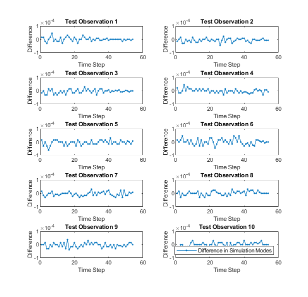
Compute the error from the PIL simulation and plot the results.

YPred_error = YPred_ref-YPred_pil;

figure('Name', 'PIL Error')
for i = 1:10
    subplot(5,2,i)
    
    plot(YPred_error(:,:,i),'.-')
    maxerror = string(max(YPred_error(:,:,i)));
    ylim([-1e-4 1e-4])
    title("Test Observation " + i)
    xlabel("Time Step")
    ylabel("Difference")
end
legend(["Difference in Simulation Modes"],'Location','southeast')

Supporting Functions

function rulExamplePlots(observationIdx,YTest,YPred)
N = numel(observationIdx);

figure
for i = 1:N
    subplot(N/2,2,i)

    plot(YTest{observationIdx(i)},'--')
    hold on
    plot(YPred{observationIdx(i)},'.-')
    hold off

    ylim([0 175])
    title("Test Observation " + observationIdx(i))
    xlabel("Time Step")
    ylabel("RUL")
end
legend(["Test Data" "Predicted"],'Location','southeast')

end

References

Saxena, Abhinav, Kai Goebel, Don Simon, and Neil Eklund. "Damage propagation modeling for aircraft engine run-to-failure simulation." In Prognostics and Health Management, 2008. PHM 2008. International Conference on, pp. 1-9. IEEE, 2008.