Estimate Conditional Mean and Variance Model

Load and Preprocess Data

Load the NASDAQ data included with Econometrics Toolbox™. Convert the daily close composite index series to a return series. For numerical stability, convert the returns to percentage returns.

load Data_EquityIdx
nasdaq = DataTable.NASDAQ;
r = 100*price2ret(nasdaq);
T = length(r);

Create Model Template

Create an AR(1) and GARCH(1,1) composite model, which has the form

where $${\epsilon }_t={\sigma }_t{z}_t$$ and $$z_t$$ is an iid standardized Gaussian process.

VarMdl = garch(1,1)

VarMdl = 
  garch with properties:

     Description: "GARCH(1,1) Conditional Variance Model (Gaussian Distribution)"
      SeriesName: "Y"
    Distribution: Name = "Gaussian"
               P: 1
               Q: 1
        Constant: NaN
           GARCH: {NaN} at lag [1]
            ARCH: {NaN} at lag [1]
          Offset: 0

Mdl = arima('ARLags',1,'Variance',VarMdl)

Mdl = 
  arima with properties:

     Description: "ARIMA(1,0,0) Model (Gaussian Distribution)"
      SeriesName: "Y"
    Distribution: Name = "Gaussian"
               P: 1
               D: 0
               Q: 0
        Constant: NaN
              AR: {NaN} at lag [1]
             SAR: {}
              MA: {}
             SMA: {}
     Seasonality: 0
            Beta: [1×0]
        Variance: [GARCH(1,1) Model]

Mdl is an arima model template for estimation. NaN-valued properties of Mdl and VarMdl correspond to unknown, estimable coefficients and variance parameters of the composite model.

Estimate Model Parameters

Fit the model to the return series r by using estimate.

EstMdl = estimate(Mdl,r);

 
    ARIMA(1,0,0) Model (Gaussian Distribution):
 
                 Value      StandardError    TStatistic      PValue  
                ________    _____________    __________    __________

    Constant    0.072632      0.018047         4.0245      5.7086e-05
    AR{1}        0.13816      0.019893          6.945      3.7845e-12

 
 
    GARCH(1,1) Conditional Variance Model (Gaussian Distribution):
 
                 Value      StandardError    TStatistic      PValue  
                ________    _____________    __________    __________

    Constant    0.022377      0.0033201        6.7399      1.5852e-11
    GARCH{1}     0.87312      0.0091019        95.927               0
    ARCH{1}      0.11865       0.008717        13.611      3.4339e-42

EstMdl is a fully specified arima model.

The estimation display shows the five estimated parameters and their corresponding standard errors (the AR(1) conditional mean model has two parameters, and the GARCH(1,1) conditional variance model has three parameters).

The fitted model (EstMdl) is

All $\mathit{t}$ statistics are greater than 2, which suggests that all parameters are statistically significant.

Dynamic models require presample observations, with which to initialize the model. If you do not specify presample observations, estimate generates them by default.

Infer Conditional Variances and Residuals

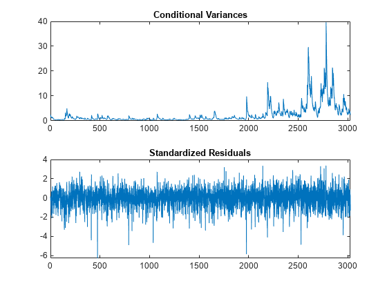
Infer and plot the conditional variances and standardized residuals. Output the loglikelihood objective function value.

[res,v,logL] = infer(EstMdl,r);

figure
subplot(2,1,1)
plot(v)
xlim([0,T])
title('Conditional Variances')

subplot(2,1,2)
plot(res./sqrt(v))
xlim([0,T])
title('Standardized Residuals')

The conditional variances increase after observation 2000. This result corresponds to the increased volatility seen in the original return series.

The standardized residuals have more large values (larger than 2 or 3 in absolute value) than expected under a standard normal distribution. This result suggests a Student's $\mathit{t}$ distribution can be more appropriate for the innovation distribution.

Fit Model With t Innovation Distribution

Create a model template from Mdl, and specify that its innovations have a Student's $\mathit{t}$ distribution.

MdlT = Mdl;
MdlT.Distribution = 't';

MdlT has one additional parameter estimate: the $\mathit{t}$ distribution degrees of freedom.

Fit the new model to the NASDAQ return series. Specify an initial value for the variance model constant term.

Variance0 = {'Constant0',0.001};
EstMdlT = estimate(MdlT,r,'Variance0',Variance0);

 
    ARIMA(1,0,0) Model (t Distribution):
 
                 Value      StandardError    TStatistic      PValue  
                ________    _____________    __________    __________

    Constant    0.093488      0.016694         5.6002      2.1414e-08
    AR{1}        0.13911      0.018857         7.3771      1.6175e-13
    DoF           7.4775       0.88261          8.472      2.4126e-17

 
 
    GARCH(1,1) Conditional Variance Model (t Distribution):
 
                 Value      StandardError    TStatistic      PValue  
                ________    _____________    __________    __________

    Constant    0.011246      0.0036305        3.0976       0.0019511
    GARCH{1}     0.90766       0.010516        86.315               0
    ARCH{1}     0.089897       0.010835        8.2966      1.0712e-16
    DoF           7.4775        0.88261         8.472      2.4126e-17

The coefficient estimates between EstMdl and EstMdlT are slightly different. The degrees of freedom estimate is relatively small (about 8), which indicates a significant departure from normality.

Compare Model Fits

Summarize the estimated models. From the summaries, obtain the number of estimated parameters and the loglikelihood objective function value from the second fit.

Summary = summarize(EstMdl);
SummaryT = summarize(EstMdlT);

numparams = Summary.NumEstimatedParameters;
numparamsT = SummaryT.NumEstimatedParameters;
logLT = SummaryT.LogLikelihood;

Compare the two model fits (Gaussian and $\mathit{t}$ innovation distribution) using the Akaike information criterion (AIC) and Bayesian information criterion (BIC).

[numparams numparamsT]

ans = 1×2

     5     6

[aic,bic] = aicbic([logL logLT],[numparams numparamsT],T)

aic = 1×2
103 ×

    9.4929    9.3807

bic = 1×2
103 ×

    9.5230    9.4168

The first model has six fitted parameters, whereas the second model has six (because it contains the $\mathit{t}$ distribution degrees of freedom). Despite this difference, both information criteria favor the model with the Student's $\mathit{t}$ innovation distribution because it yields smaller AIC and BIC values than the model with Gaussian innovations.