Volatility Modeling for Soft Commodities

This example uses:

This example demonstrates a diverse set of statistical methods, machine learning techniques, and time-series models that you can apply broadly in the field of volatility modeling. Specifically, this example focuses on the analysis, modeling, and forecasting of volatility within the context of soft commodities.

Soft commodities refer to agricultural products that are grown rather than mined or extracted. These commodities are typically perishable and have a shorter shelf life compared to hard commodities like metals or energy resources. Soft commodities are highly influenced by uncertainties arising from climate change-induced shifts in weather patterns, both in the short and the long term. With the growing magnitude of these uncertainties, volatility modeling is becoming increasingly crucial. Practitioners are actively seeking to enhance their ability to forecast market responses to climate change impacts, emphasizing the importance of volatility modeling for soft commodities.

The goal of this example is to provide insights into the patterns and dynamics of volatility in the soft commodities market and to improve the accuracy of volatility forecasts. With more accurate forecasts, market participants can make more informed decisions to effectively manage risk in the face of climate-related uncertainties.

Import Commodity Price Data

Import the historical price data for a set of commodities and then organize and process the data into a suitable form for subsequent analysis. The data is sourced from the World Bank's monthly commodity price data set. The data comprises monthly commodity prices for a diverse collection of soft commodities.

Download the data set (CMO-Historical-Data-Monthly.xlsx) for the World Bank's monthly commodity price data set [1] by using the webread function and the local function importCommodityData.

dataURL = "https://thedocs.worldbank.org/en/doc/5d903e848db1d1b83e0ec8f744e55570-0350012021/related/CMO-Historical-Data-Monthly.xlsx";
webOpts = weboptions("ContentReader", @importCommodityData);
Prices = webread(dataURL, webOpts);

Process Raw Commodity Price Data

Convert the dates to datetime values and then convert the resulting table to a timetable.

Prices.Date = datetime(Prices.Date, ...
    "InputFormat", "yyyy'M'MM", ...
    "Format", "MMM yyyy");
Prices = table2timetable(Prices);

Associate high-level classes with each commodity. This example uses these high-level classes to extract the soft commodities from the larger data set.

commodityClasses = categorical([repmat("Energy", 1, 10), ...
    repmat("Beverages", 1, 7), ...
    repmat("Oils and Meals", 1, 11), ...
    repmat("Grains", 1, 9), ...
    repmat("Other Food", 1, 10), ...
    repmat("Raw Materials", 1, 9), ...
    repmat("Fertilizers", 1, 5), ...
    repmat("Metals and Minerals", 1, 7), ...
    repmat("Precious Metals", 1, 3)] );

Prices = addprop(Prices, "CommodityClass", "variable");
Prices.Properties.CustomProperties.CommodityClass = commodityClasses;

Similarly, associate a hard and soft label with each commodity, using the previously defined commodity classes.

commodityTypes = categorical(repmat("Soft", 1, width(Prices)));
hardClasses = categorical(["Energy", "Fertilizers", "Metals and Minerals", "Precious Metals"]);
hardIdx = ismember(commodityClasses, hardClasses);
commodityTypes(hardIdx) = "Hard";

Prices = addprop( Prices, "CommodityType", "variable" );
Prices.Properties.CustomProperties.CommodityType = commodityTypes;

Create Portfolio of Soft Commodities

Extract the soft commodities that have no missing data for the entire period.

soft = Prices.Properties.CustomProperties.CommodityType == "Soft";
intact = all(~ismissing(Prices));
Prices = Prices(:, soft & intact);

Preview the soft commodity price data.

disp(head(Prices))

      Date      Cocoa     Coffee, Arabica    Coffee, Robusta    Tea, avg 3 auctions    Tea, Colombo    Tea, Kolkata    Tea, Mombasa    Coconut oil    Groundnut oil **    Palm oil    Soybeans    Soybean oil    Soybean meal    Maize    Rice, Thai 5%    Wheat, US HRW    Banana, US    Orange    Beef **    Chicken **    Sugar, EU    Sugar, US    Sugar, world    Tobacco, US import u.v.    Logs, Malaysian    Sawnwood, Malaysian    Cotton, A Index    Rubber, RSS3
    ________    ______    _______________    _______________    ___________________    ____________    ____________    ____________    ___________    ________________    ________    ________    ___________    ____________    _____    _____________    _____________    __________    ______    _______    __________    _________    _________    ____________    _______________________    _______________    ___________________    _______________    ____________

    Jan 1960     0.634        0.9409             0.69686              1.0297              0.9303          1.1214          1.0374           390              334             233          94           204            91.9         45         104.45            59.89         0.14308      0.1151    0.7055      0.29737       0.12236      0.11684        0.0666               1736.9                  31.94               149.17               0.6486            0.8223   
    Feb 1960     0.608        0.9469             0.68871              1.0297              0.9303          1.1214          1.0374           379              341             229          91           201            86.7         44         103.54            60.99         0.14308      0.1092    0.7121      0.29742       0.12236      0.11905        0.0679               1736.9                  31.94               149.17               0.6453            0.8289   
    Mar 1960    0.5789        0.9281             0.68871              1.0297              0.9303          1.1214          1.0374           361              338             225          92           201            84.1         45         103.79            61.73         0.14308      0.1319    0.7694      0.29783       0.12236      0.12125        0.0683               1736.9                  31.94               149.17               0.6464            0.8576   
    Apr 1960    0.5983        0.9303             0.68452              1.0297              0.9303          1.1214          1.0374           338              333             225          93           207            86.7         45         100.97            60.99         0.14308      0.1363    0.8378      0.29902       0.12236      0.12346        0.0681               1736.9                  31.94               149.17               0.6435            0.8642   
    May 1960    0.6001          0.92             0.69069              1.0297              0.9303          1.1214          1.0374           321              335             225          93           209            81.5         48         102.15            57.69           0.149      0.1444    0.7562      0.29903       0.12236      0.12125        0.0683               1736.9                  31.94               149.17               0.6468            0.9281   
    Jun 1960    0.5944        0.9123             0.69686              1.0297              0.9303          1.1214          1.0374           287              334             219          91           218            80.3         47         103.13            55.48           0.149      0.1385    0.7077      0.29964       0.12236      0.12566        0.0666               1736.9                  31.94               149.17               0.6559            0.8929   
    Jul 1960    0.6045         0.916             0.69069              1.0297              0.9303          1.1214          1.0374           298              336             221          92           224            77.7         47         102.05            54.75           0.149      0.1292    0.7474      0.30002       0.12236      0.13228        0.0728               1736.9                  31.94               149.17               0.6572             0.787   
    Aug 1960    0.5882        0.9292             0.69885              1.0297              0.9303          1.1214          1.0374           292              336             225          93           237            77.7         47         109.71            55.12         0.12699      0.1292    0.7826      0.30083       0.12236      0.12787        0.0741               1736.9                  31.94               149.17               0.6534            0.7209

Adjust Soft Commodity Price Data

The price data is in nominal US dollars. You can use an external inflation metric to adjust the nominal commodity prices and approximate a real (inflation-adjusted) price series.

First, obtain the external inflation metric (a consumer price index) over the same date range as observed in the commodity prices.

You obtain the consumer price index series CUUR0000SA0R from the Bureau of Labor Statistics [2]. Use this consumer price series index to create the inflation timetable.

[startDate, endDate] = bounds(Prices.Date);
inflation = readtimetable("CUUR0000SA0R.csv");
inflation = inflation(timerange(startDate, endDate), :);

Adjust the data to reflect January 2022 US dollars. First, rebase the inflation index so that January 2022 has value 1.

rebaseDate = datetime(2022, 01, 01);
inflation{:, 1} = inflation{:, 1} / inflation{rebaseDate, 1};

Determine the common dates between the commodity series and the inflation metric.

[inflationIdx, commodityIdx] = intersect(inflation.DATE, Prices.Date);

Adjust the commodity prices over this time range using the inflation metric.

Prices = Prices(commodityIdx, :);
inflation = inflation{inflationIdx, :};
Prices.Variables = Prices.Variables .* inflation;

Visualize Adjusted Commodity Price Data

Plot each price series for soft commodities over time.

commodityNames = string(Prices.Properties.VariableNames);

figure

tiledlayout(8,4, "TileSpacing", "tight")

for commodity = 1:width(Prices)
    nexttile
    plot(Prices.Date, Prices{:, commodity})
    title(commodityNames(commodity))   
    axis off
end

sgtitle("Commodity Prices")

Compute Commodity Price Returns

To further analyze the data in this example, you must work with the commodity price returns rather than the adjusted commodity prices. Use tick2ret to convert the adjusted commodity prices $P_{t}$ to the return series $R_{t}$ as follows:

$R_{t} = \frac{P_{t + 1}}{P_{t}} - 1, t = 1, 2, 3, \dots$

Returns = tick2ret(Prices);

Visualize Commodity Price Returns

Plot each return series for soft commodities over time.

figure
tiledlayout(8,4, "TileSpacing", "tight")

for commodity = 1:width(Returns)
    nexttile
    plot(Returns.Date, Returns{:, commodity})
    title(commodityNames(commodity))
    axis off
end

sgtitle("Commodity Returns")

Decompose Prices and Cluster Commodities

Decompose each commodity price series into a long-term trend, a seasonal component, and an irregular (or business cycle) component. This operation is an additive decomposition:

$P_{t} = L_{t} + S_{t} + C_{t}, t = 1, 2, 3, \dots,$

where:

$P_{t}$ is the commodity price series.
$L_{t}$ is the long-term trend.
$S_{t}$ is the seasonal component (which may be the sum of multiple seasonal trends).
$C_{t}$ is the irregular component.

Based on the relative similarity of the irregular components of the commodity price series, you can cluster the commodities into groups using unsupervised machine learning techniques.

Decompose Commodity Prices

Preallocate variables for the soft commodity series components.

numObservations = height( Prices );
numCommodities = width( Prices );

longTermComponent = NaN( numObservations, numCommodities );
seasonalComponent = NaN( numObservations, numCommodities );
irregularComponent = NaN( numObservations, numCommodities );
regularComponent = NaN( numObservations, numCommodities );

Create tiled layouts for the visualization. You can visualize the trend components (for example, the sum of $L_{t}$ and $S_{t}$ ) separately from the irregular components ( $C_{t}$ ).

figure
tlTrend = tiledlayout(8,4, "TileSpacing", "tight");
title( tlTrend, "Trend Components" )

figure
tlIrregular = tiledlayout(8,4, "TileSpacing", "tight");
title( tlIrregular, "Irregular Components")

For each soft commodity price series, perform the trend decomposition by using trenddecomp.

for k = 1:numCommodities

    % Decompose the price series and store the results. This process might identify 
    % more than one seasonal component, so sum the resulting matrix of seasonal 
    % components to obtain the overall seasonal trend.
    [L, S, C] = trenddecomp( Prices{:, k} );
    longTermComponent(:, k) = L;
    seasonalComponent(:, k) = sum( S, 2 );
    irregularComponent(:, k) = C;
    regularComponent(:, k) = longTermComponent(:, k) + seasonalComponent(:, k);

    % Add the components to the visualization.
    nexttile(tlTrend)
    plot(Prices.Date, regularComponent(:, k) )
    title(commodityNames(k))
    axis off

    nexttile(tlIrregular)
    plot(Prices.Date, irregularComponent(:, k))
    title(commodityNames(k))
    axis off

end

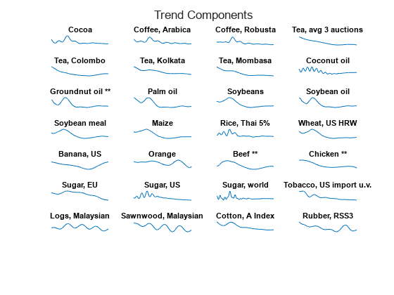
From the trend decomposition and by inspecting the series $L_{t} + S_{t}$ for each commodity, you can see that most commodities show a long-term decrease in price over recent decades, followed by a more recent upturn in the price.

Some exceptions, such as the series Sugar, EU, show a long-term downward trend.

Some commodities also appear to have gone through periods of high seasonal volatility, such as the two coffee price series. Banana and orange prices appear to be more susceptible to seasonal volatility. Chicken prices exhibit seasonal volatility that has increased in the last few years.

Cluster Commodities Based on Similarity in Irregular Component

After removing the long-term and seasonal components from the price series, you are left with the irregular component $C_{t}$ , given by

$C_{t} = P_{t} - L_{t} - S_{t}$ .

The $C_{t}$ component represents the business cycle component in the soft commodity time series and this series is affected by short-term market conditions. This component provides a fairer basis for comparing the soft commodity prices because both the long-term price trends and the seasonal trends are removed.

Compute the pairwise distances between the irregular components using the correlation distance metric $d$ . This metric is defined by

$d (s_{1}, s_{2}) = 1 - ρ (s_{1}, s_{2})$ , where $ρ (s_{1}, s_{2})$ is the linear correlation coefficient between the two time series $s_{1}$ and $s_{2}$ .

irregularCorrDistances = pdist( irregularComponent.', "correlation" );

Use linkage to perform hierarchical clustering using the correlation distances. The complete method uses the largest distance between commodities in the two clusters.

irregularComponentLinkage = linkage( irregularCorrDistances, "complete" );

Create a dendrogram to visualize the linkage.

figure
h = dendrogram( irregularComponentLinkage, numCommodities, ...
    "Labels", commodityNames, ...
    "ColorThreshold", 1.2 );
ylabel( "Dissimilarity" )
title( "Commodity Price Series Clustering" )
subtitle( "Irregular Component Correlation Distance" )
set( h, "LineWidth", 2 )
xtickangle( 45 )
grid( "on" )
box( "on" )

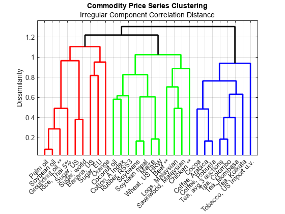
Figure contains an axes object. The axes object with title Commodity Price Series Clustering, ylabel Dissimilarity contains 27 objects of type line.

Cluster the commodities into five groups based on their similarity obtained from this dendrogram.

numClusters = 3;
Group = cluster( irregularComponentLinkage, "maxclust", numClusters );
Commodity = string( commodityNames.' );
clusteredCommodities = table( Commodity, Group );
commoditiesByCluster = sortrows( clusteredCommodities, "Group" );
disp( commoditiesByCluster )

            Commodity            Group
    _________________________    _____

    "Coconut oil"                  1  
    "Soybeans"                     1  
    "Soybean meal"                 1  
    "Maize"                        1  
    "Wheat, US HRW"                1  
    "Beef **"                      1  
    "Chicken **"                   1  
    "Logs, Malaysian"              1  
    "Sawnwood, Malaysian"          1  
    "Cotton, A Index"              1  
    "Rubber, RSS3"                 1  
    "Groundnut oil **"             2  
    "Palm oil"                     2  
    "Soybean oil"                  2  
    "Rice, Thai 5%"                2  
    "Banana, US"                   2  
    "Orange"                       2  
    "Sugar, EU"                    2  
    "Sugar, US"                    2  
    "Sugar, world"                 2  
    "Cocoa"                        3  
    "Coffee, Arabica"              3  
    "Coffee, Robusta"              3  
    "Tea, avg 3 auctions"          3  
    "Tea, Colombo"                 3  
    "Tea, Kolkata"                 3  
    "Tea, Mombasa"                 3  
    "Tobacco, US import u.v."      3

Cluster Commodities Based on Similarity in Regular Component

The regular component is the sum of the long-term and seasonal trends $L_{t} + S_{t}$ , and is equal to $P_{t} - C_{t}$ , the commodity price series without its irregular (business cycle) component.

Evaluate the pairwise distances and the corresponding linkage.

regularCorrDistances = pdist( regularComponent.', "correlation" );
regularComponentLinkage = linkage( regularCorrDistances, "complete" );

Create a dendrogram to visualize the linkage, and then select a threshold to achieve three clusters.

figure
h = dendrogram( regularComponentLinkage, numCommodities, ...
    "Labels", commodityNames, ...
    "ColorThreshold", 0.8 );
ylabel( "Dissimilarity" )
title( "Commodity Price Series Clustering" )
subtitle( "Regular Component Correlation Distance" )
set( h, "LineWidth", 2 )
xtickangle( 45 )
grid( "on" )
box( "on" )

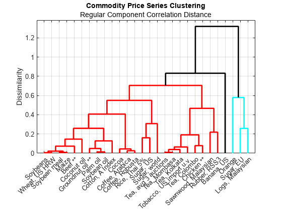
Figure contains an axes object. The axes object with title Commodity Price Series Clustering, ylabel Dissimilarity contains 27 objects of type line.

You might expect the volatility in the commodities to manifest itself in the irregular component, rather than the regular component. For this reason, continue with the clusters identified by performing hierarchical clustering on the irregular components of the commodity price series. However, clustering on the regular components provides a useful grouping of the commodities based on their combined long-term and seasonal trends. From the dendrogram, you can see that both oranges and bananas have a dissimilar regular profile to the other commodities.

Visualize Clusters in 3D

Embed the commodities in a lower-dimensional space by using classical multi-dimensional scaling using cmdscale.

lowerDim = 3;
Y = cmdscale( irregularCorrDistances, lowerDim );

Visualize the embedding. Add the convex hull of each group using convhull to illustrate the different groupings in 3-dimensional space.

figure
view( 3 )
clusterColors = hsv( numClusters );
colormap( clusterColors )
hold( "on" )

for k = 1:numClusters
    % Extract coordinate data for the current group.
    idx = clusteredCommodities.Group == k;
    clusterx = Y(idx, 1);
    clustery = Y(idx, 2);
    clusterz = Y(idx, 3);
    color = clusterColors(k, :);
    % Evaluate the convex hull.
    ch = convhull( clusterx, clustery, clusterz );
    % Visualize the convex hull, its vertices (the commodities), and create
    % text labels.
    trisurf( ch, clusterx, clustery, clusterz, ...
        "FaceColor", clusterColors(k, :), ...
        "FaceAlpha", 0.25, ...
        "EdgeColor", "none", ...
        "HandleVisibility", "off" )
    scatter3( clusterx, clustery, clusterz, ...
        [], clusterColors(k, :), "filled", "DisplayName", "Cluster " + k )
    text( clusterx, clustery, clusterz, ...
        clusteredCommodities.Commodity(idx), "Rotation", 10 )
end

xticks( [] )
yticks( [] )
zticks( [] )
title( "Commodity Clusters in 3D Space" )
lg = legend( "Location", "eastoutside" );
title( lg, "Commodity Cluster" )

Figure contains an axes object. The axes object with title Commodity Clusters in 3D Space contains 31 objects of type scatter, text. These objects represent Cluster 1, Cluster 2, Cluster 3.

Estimate Nonparametric Volatility

Obtain a nonparametric volatility estimate for each soft commodity series using an exponentially weighted moving average (EWMA).

To estimate the underlying volatility of a time series using an EWMA model, let ${r_{n}}$ denote the sequence of commodity returns and let ${y_{n}}$ be the sequence of EWMA estimates for the instantaneous variance. The difference equation for computing the sequence ${y_{n}}$ is as follows:

$y_{1} = r_{1}^{2}, y_{n} = λ y_{n - 1} + (1 - λ) r_{n}^{2}, λ \in [0, 1], n \geq 2$

Here, $λ$ is a scalar smoothing parameter chosen from the interval $[0, 1]$ .
In many typical applications, $0.90 \leq λ \leq 0.99$ . In this example, you take $λ = 0.94$ .
As $λ$ increases, the influence of the previous moving average estimate ( $y_{n - 1}$ ) on the current variance estimate ( $y_{n}$ ) increases, and the influence of the current squared return ( $r_{n}^{2}$ ) decreases.
If $λ$ is close to 1, then the influence of the current squared return value $r_{n}^{2}$ is negligible in the moving average and $y_{n - 1}$ dominates. If $λ$ is close to 0, then the current squared return value $r_{n}^{2}$ dominates and $y_{n - 1}$ is negligible.

This example uses the square of the commodity returns in the EWMA computation because you estimate the instantaneous variance of the portfolio return series, from which you take the square root to obtain estimates for the instantaneous volatility (standard deviation).

Compute Exponentially Weighted Moving Averages

Define the smoothing parameter $λ$ .

lambda = 0.94;

Standard form for a filter in MATLAB® is the following:

$a_{0} y_{n} = b_{0} x_{n} + b_{1} x_{n - 1} + \dots + b_{k} x_{n - k} - a_{1} y_{n - 1} - \dots - a_{n - ℓ} y_{n - ℓ}$

where $a = [a_{0}, a_{1}, a_{2}, a_{n - ℓ}]$ and $b = [b_{0}, b_{1}, \dots, b_{k}]$ are the filter coefficients. For more information, see filter.

Write the EWMA filter coefficients in standard form:

$1 y_{n} + (- λ) y_{n - 1} = (1 - λ) r_{n}^{2}$

Here, you have $a = [1, - λ]$ and $b = [1 - λ] = 1 - λ$ .

a = [1, -lambda];
b = 1 - lambda;

Compute the instantaneous variance and volatility estimates.

instantVariance = filter(b, a, Returns.Variables.^2);
InferredVolatility = sqrt( instantVariance );

Create a timetable containing the estimated volatilities.

InferredVolatility = array2timetable( InferredVolatility, ...
    "VariableNames", commodityNames, ...
    "RowTimes", Returns.Date );
InferredVolatility.Properties.DimensionNames(1) = "Date";

Visualize Estimated Volatility Series

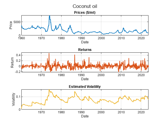
Select one of the soft commodities and visualize that commodity's price series, return series, and the inferred volatility.

chosenCommodity = commodityNames(8);

figure
tiledlayout( 3, 1 )
sgtitle( chosenCommodity )
corder = colororder();

nexttile
plot( Prices.Date, Prices.(chosenCommodity{1}), ...
    "LineWidth", 1.5, "Color", corder(1, :) )
xlabel( "Date" )
ylabel( "Price" )
units = Prices.Properties.VariableUnits(chosenCommodity);
title( "Prices " + units )
grid on

nexttile
plot( Returns.Date, Returns.(chosenCommodity{1}), ...
    "LineWidth", 1.5, "Color", corder(2, :) )
xlabel( "Date" )
ylabel( "Return" )
title( "Returns" )
grid on

nexttile
plot( InferredVolatility.Date, InferredVolatility.(chosenCommodity{1}), ...
    "LineWidth", 1.5, "Color", corder(3, :) )
xlabel( "Date" )
ylabel( "Volatility" )
title( "Estimated Volatility" )
grid on

Figure contains 3 axes objects. Axes object 1 with title Prices ($/mt), xlabel Date, ylabel Price contains an object of type line. Axes object 2 with title Returns, xlabel Date, ylabel Return contains an object of type line. Axes object 3 with title Estimated Volatility, xlabel Date, ylabel Volatility contains an object of type line.

Use Estimated Volatility to Perform Factor Analysis on Commodities

Applying factor analysis is another technique for grouping the commodities into clusters, based on the estimated volatility profiles.

Factor analysis assumes the existence of a certain number of hidden or latent factors underlying the data. If you hypothesize that the volatility in the soft commodities is driven by a smaller number of latent factors (such as external market conditions), then factor analysis provides one approach for understanding these hidden factors. For more information on factor analysis, see factoran.

numLatentFactors = 3;
loadings = factoran( InferredVolatility.Variables, numLatentFactors );

Visualize the factor loadings by using heatmap.

figure
heatmap( 1:numLatentFactors, commodityNames, loadings, ...
    "Colormap", turbo, ...
    "ColorLimits", [-1, 1] )
xlabel( "Latent Factor" )
title( "Volatility Factor Analysis" )

Figure contains an object of type heatmap. The chart of type heatmap has title Volatility Factor Analysis.

Using heatmap again, visualize the strongest association with each latent factor for each factor.

maxIdx = double( loadings == max( loadings, [], 2 ) );
figure
heatmap( 1:numLatentFactors, commodityNames, maxIdx, ...
    "Colormap", turbo, ...
    "ColorLimits", [-1, 1] )
xlabel( "Latent Factor" )
title( "Maximum Factor Loadings" )

Figure contains an object of type heatmap. The chart of type heatmap has title Maximum Factor Loadings.

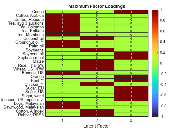
Looking at the Maximum Factor Loadings heatmap, you can see:

Coffee, tea, groundnut oil, palm oil, bananas, and wood have a strong association with latent factor 1.
Coconut oil, soybeans, maize, rice, wheat, chicken, cotton, and rubber have a strong association with latent factor 2.
Latent factor 3 is associated with cocoa, soybean oil, soybean meal, oranges, beef, shrimps, sugar, and tobacco.
The strongest negative association in the loadings matrix is chicken with latent factor 3. Other loadings for chicken are relatively low, indicating that chicken volatility is an outlier in this data set, as you can also observe by using other methods.

Estimate Model-Based Volatility

One disadvantage of using the exponentially weighted moving average for volatility estimation is that it does not provide volatility forecasts. However, you can use a model-based approach to create volatility forecasts. This example uses arima (Econometrics Toolbox) and garch (Econometrics Toolbox) time-series models.

Compute Principal Components of Inferred Volatility

First, use normalize on the volatility series and store the mean and standard deviation for later use.

[normalizedVolatility, mu, sigma] = normalize( InferredVolatility.Variables, "zscore" );

Next, compute the principal components by using pca.

[coeffs, scores, eigVals] = pca( normalizedVolatility );

Visualize the eigenvalues of the covariance matrix of the normalized volatilities.

figure
plot( eigVals, "o-", "LineWidth", 2 )
xlabel( "Principal Component" )
ylabel( "Eigenvalue" )
title( "Principal Component Eigenvalues" )
grid( "on" )

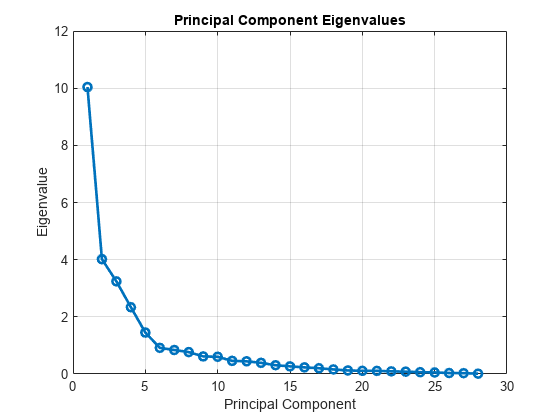
Figure contains an axes object. The axes object with title Principal Component Eigenvalues, xlabel Principal Component, ylabel Eigenvalue contains an object of type line.

You can see that most of the variance in the data is captured by the first few principal components.

Visualize the first two principal components.

numComponents = 2;

figure
tiledlayout( "flow" )

for k = 1:numComponents
    nexttile
    plot( InferredVolatility.Date, scores(:, k ) )
    title( "Component: " + k )
    grid( "on" )
end

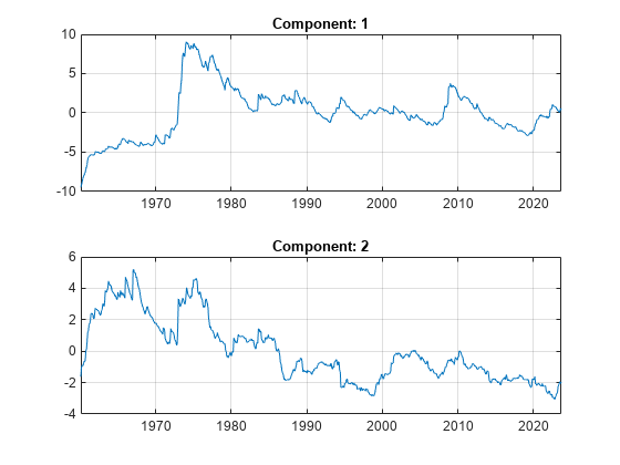
Figure contains 2 axes objects. Axes object 1 with title Component: 1 contains an object of type line. Axes object 2 with title Component: 2 contains an object of type line.

Model Principal Components

Rather than creating many separate time-series models for each soft commodity, you can take an efficient approach by building models for only the first few principal components. You can then back-transform forecasts from these models into the original domain.

Create and fit an arima (Econometrics Toolbox) time-series model for the first principal component.

firstComponent = scores(:, 1);

firstComponentModel = arima( "ARLags", 1, ...
    "MALags", 1, ...
    "Distribution", "t", ...
    "Variance", garch( 1, 1 ) );
firstComponentModel = estimate( firstComponentModel, firstComponent );

 
    ARIMA(1,0,1) Model (t Distribution):
 
                  Value      StandardError    TStatistic      PValue  
                _________    _____________    __________    __________

    Constant    -0.063238       0.006214       -10.177      2.5191e-24
    AR{1}         0.98215      0.0019302        508.82               0
    MA{1}         0.15671       0.031714        4.9412      7.7629e-07
    DoF            2.5091        0.24115        10.405      2.3521e-25

 
 
    GARCH(1,1) Conditional Variance Model (t Distribution):
 
                 Value      StandardError    TStatistic      PValue  
                ________    _____________    __________    __________

    Constant    0.013581      0.0062827        2.1617        0.030644
    GARCH{1}     0.69036       0.083993        8.2193      2.0472e-16
    ARCH{1}      0.18852       0.089543        2.1053        0.035264
    DoF           2.5091        0.24115        10.405      2.3521e-25

Create and fit an arima (Econometrics Toolbox) time-series model for the second principal component.

secondComponent = scores(:, 2);
secondComponentModel = arima("ARLags", 1, ...
    "MALags", 1, ...
    "Distribution", "t", ...
    "Variance", garch( "ARCHLags", 1, ...
    "Constant", 0.01, ...
    "GARCHLags", 1 ) );
secondComponentModel = estimate( secondComponentModel, secondComponent );

 
    ARIMA(1,0,1) Model (t Distribution):
 
                  Value      StandardError    TStatistic      PValue   
                _________    _____________    __________    ___________

    Constant    -0.025173      0.0043829       -5.7433       9.2839e-09
    AR{1}         0.98224       0.002459        399.45                0
    MA{1}        0.077561       0.025207        3.0769        0.0020913
    DoF            2.1625       0.086605         24.97      1.3059e-137

 
 
    GARCH(1,1) Conditional Variance Model (t Distribution):
 
                 Value      StandardError    TStatistic      PValue   
                ________    _____________    __________    ___________

    Constant        0.01             0            Inf                0
    GARCH{1}     0.86678       0.05892         14.711       5.4685e-49
    ARCH{1}     0.084508       0.04304         1.9635         0.049593
    DoF           2.1625      0.086605          24.97      1.3059e-137

Create Simulated Component Values from Fitted Models

Use simulate (Econometrics Toolbox) to create the simulated component values from the fitted models.

numForecastSteps = 60;
simFirstComponent = simulate( firstComponentModel, numForecastSteps, "Y0", firstComponent );
simSecondComponent = simulate( secondComponentModel, numForecastSteps, "Y0", secondComponent );
simComponents = [simFirstComponent, simSecondComponent];

Back-Transform Simulated Component Values

Transform the simulation results in the principal component domain back to the original volatility domain, adjusting for the normalization step performed in Compute Principal Components of Inferred Volatility. Since you have modeled only the first two principal components, this transformation is an approximation to the volatility. Modeling more of the principal components would lead to a more accurate volatility approximation at the cost of more modeling, simulation, and execution time.

approxVolatility = mu + sigma .* (simComponents * coeffs(:, 1:2).');
approxVolatility = [InferredVolatility{end, :}; approxVolatility];

Convert the volatility approximations to the timetable format.

simDates = InferredVolatility.Date(end) + calmonths(0:numForecastSteps).';
approxVolatility = array2timetable( approxVolatility, ...
    "RowTimes", simDates, "VariableNames", commodityNames );
approxVolatility.Properties.DimensionNames(1) = "Date";

Visualize Volatility Simulation Results

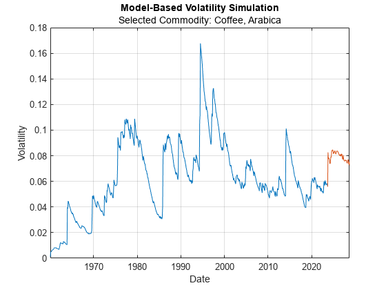
In the Model-Based Volatility Simulation plot, the blue line indicates historical data and the red line indicates the simulated volatility moving into the future.

selectedCommodity = commodityNames(2);

figure
plot( InferredVolatility.Date, InferredVolatility.(selectedCommodity) )
hold on
plot( approxVolatility.Date, approxVolatility.(selectedCommodity) )
xlabel( "Date" )
ylabel( "Volatility" )
title( "Model-Based Volatility Simulation" )
subtitle( "Selected Commodity: " + selectedCommodity )
grid on

Figure contains an axes object. The axes object with title Model-Based Volatility Simulation, xlabel Date, ylabel Volatility contains 2 objects of type line.

References

[1] The World Bank: Commodity Monthly Prices, located at: https://www.worldbank.org/en/research/commodity-markets and licensed under CC BY 4.0 Deed | Attribution 4.0 International | Creative Commons.

[2] U.S. Bureau of Labor Statistics, Consumer Price Index for All Urban Consumers: Purchasing Power of the Consumer Dollar in U.S. City Average [CUUR0000SA0R]. Available at https://beta.bls.gov/dataViewer/view/timeseries/CUUR0000SA0R. Data provided by the U.S. Bureau of Labor Statistics through the BLS Data Viewer at BLS.gov. BLS.gov cannot vouch for the data or analyses derived from these data after the data have been retrieved from BLS.gov.

Local Functions

% Import the commodity data.
function Prices = importCommodityData(filename)

% Detect the import options for the file CMO-Historical-Data-Monthly.xlsx.
opts = detectImportOptions(filename, ...
    "Sheet", "Monthly Prices", ...
    "VariableNamingRule", "preserve", ...
    "TextType", "string");

% Rename the first variable to Date.
opts.VariableNames = replace(opts.VariableNames, "Var1", "Date");

% Ensure that all variables apart from the first are numeric.
numVars = length(opts.VariableTypes);
opts.VariableTypes = ["string", repmat("double", 1, numVars - 1)];

% Ensure that the variable units are imported in addition to the data.
opts.VariableUnitsRange = "A6";

% Import the data.
Prices = readtable(filename, opts);

end % importCommodityData