Forecast VAR Model
This example shows how to use forecast to forecast a VAR model.
forecast enables you to generate MMSE forecasts with error estimates. forecast requires:
A fully-specified model (for example,
EstMdlin what follows)The number of periods for the forecast (for example,
numperiodsin what follows)A presample time series (e.g.,
Y(end-3:end,:)in what follows)
forecast optionally takes:
An exogenous data series
Extra paths
Load the Data_USEconModel data set. This example uses two time series: the logarithm of real GDP, and the real 3-month T-bill rate, both differenced to be approximately stationary. Suppose that a VAR(4) model is appropriate to describe the time series.
load Data_USEconModel
DEF = log(DataTimeTable.CPIAUCSL);
GDP = log(DataTimeTable.GDP);
rGDP = diff(GDP - DEF); % Real GDP is GDP - deflation
TB3 = 0.01*DataTimeTable.TB3MS;
dDEF = 4*diff(DEF); % Scaling
rTB3 = TB3(2:end) - dDEF; % Real interest is deflated
Y = [rGDP,rTB3];
Fit a VAR(4) model specification:
Mdl = varm(2,4);
Mdl.SeriesNames = {'Transformed real GDP','Transformed real 3-mo T-bill rate'};
EstMdl = estimate(Mdl,Y);
Predict the evolution of the time series:
numperiods = 21;
FDates = dateshift(DataTimeTable.Time(end),'end','quarter',1:numperiods);
[Forecast,ForecastMSE] = forecast(EstMdl,numperiods,Y(end-3:end,:));
Extract the main diagonal elements from the matrices in each cell of ForecastMSE. Apply the square root of the result to obtain standard errors.
extractMSE = @(x)diag(x)';
MSE = cellfun(extractMSE,ForecastMSE,'UniformOutput',false);
SE = sqrt(cell2mat(MSE));
Estimate approximate 95% forecast intervals for each response series.
ForecastFI = zeros(numperiods,Mdl.NumSeries,2);

ForecastFI(:,:,1) = Forecast - 2*SE;
ForecastFI(:,:,2) = Forecast + 2*SE;
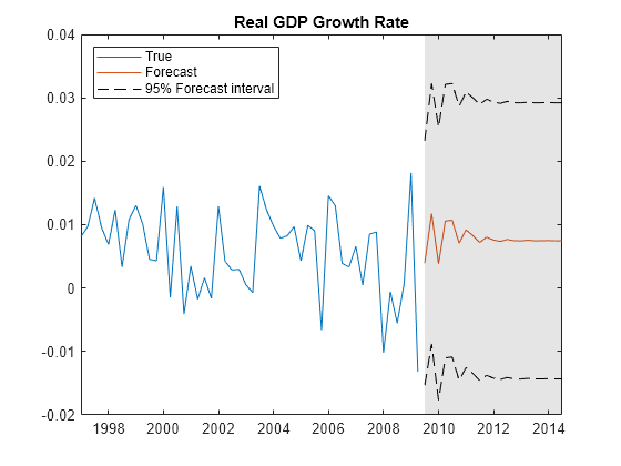
Plot the forecasts and the data.
figure
h1 = plot(DataTimeTable.Time((end-49):end),Y((end-49):end,1));
hold on
h2 = plot(FDates,Forecast(:,1));
h3 = plot(FDates,ForecastFI(:,1,1),'k--');
plot(FDates,ForecastFI(:,1,2),'k--');
title('Real GDP Growth Rate')
h = gca;
fill([FDates(1) h.XLim([2 2]) FDates(1)],h.YLim([1 1 2 2]),'k',...
    'FaceAlpha',0.1,'EdgeColor','none');
legend([h1 h2 h3],'True','Forecast','95% Forecast interval',...
    'Location','northwest')
hold off

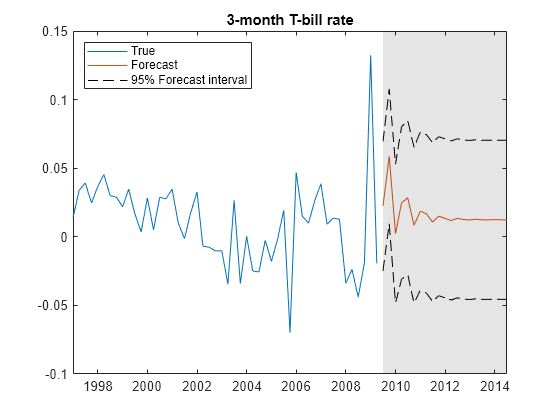
figure
h1 = plot(DataTimeTable.Time((end-49):end),Y((end-49):end,2));
hold on
h2 = plot(FDates,Forecast(:,2));
h3 = plot(FDates,ForecastFI(:,2,1),'k--');
plot(FDates,ForecastFI(:,2,2),'k--');
title('3-month T-bill rate')
h = gca;
fill([FDates(1) h.XLim([2 2]) FDates(1)],h.YLim([1 1 2 2]),'k',...
    'FaceAlpha',0.1,'EdgeColor','none');
legend([h1 h2 h3],'True','Forecast','95% Forecast interval',...
    'Location','northwest')
hold off
