varm
Create vector autoregression (VAR) model
Description
The varm
function returns a varm
object specifying the functional form and storing the parameter values of a p-order, stationary, multivariate vector autoregression model (VAR(p)) model.
The key components of a varm
object include the number of time series (response-variable dimensionality) and the order of the multivariate autoregressive polynomial (p) because they completely specify the model structure. Other model components include a regression component to associate the same exogenous predictor variables to each response series, and constant and time trend terms. Given the response-variable dimensionality and p, all coefficient matrices and innovation-distribution parameters are unknown and estimable unless you specify their values.
To estimate models containing unknown parameter values, pass the model and data to
estimate
. To work with an estimated or fully
specified varm
model object, pass it to an object
function. Alternatively, you can create and work with varm
model objects interactively by using Econometric
Modeler.
Creation
Description
creates a VAR(0) model composed of one response series.Mdl
= varm
creates a VAR(Mdl
= varm(numseries
,numlags
)numlags
) model composed of numseries
response series. The maximum nonzero lag is numlags
. All lags have numseries
-by-numseries
coefficient matrices composed of NaN
values.
This shorthand syntax allows for easy model template creation. The model template is suited for unrestricted parameter estimation, that is, estimation without parameter equality constraints. After you create a model, you can alter property values using dot notation.
sets properties or additional options using name-value pair arguments. Enclose each name in quotes. For example, Mdl
= varm(Name,Value
)'Lags',[1 4],'AR',AR
specifies the two autoregressive coefficient matrices in AR
at lags 1
and 4
.
This longhand syntax allows for creating more flexible models. varm
infers the number of series (NumSeries
) and autoregressive polynomial degree (P
) from the properties that you set. Therefore, property values that correspond to the number of series or autoregressive polynomial degree must be consistent with each other.
Input Arguments
The shorthand syntax provides an easy way for you to create model templates that are suitable for unrestricted parameter estimation. For example, to create a VAR(2) model composed of three response series, enter:
Mdl = varm(3,2);
numseries
— Number of time series m
1
(default) | positive integer
Number of time series m, specified as a positive integer. numseries
specifies the dimensionality of the multivariate response variable yt and innovation εt.
numseries
sets the NumSeries
property.
Data Types: double
numlags
— Number of lagged responses
nonnegative integer
Number of lagged responses to include in the model, specified as a nonnegative integer. The resulting model is a VAR(numlags
) model. All lags have numseries
-by-numseries
coefficient matrices composed of NaN
values.
Data Types: double
Specify optional pairs of arguments as
Name1=Value1,...,NameN=ValueN
, where Name
is
the argument name and Value
is the corresponding value.
Name-value arguments must appear after other arguments, but the order of the
pairs does not matter.
Before R2021a, use commas to separate each name and value, and enclose
Name
in quotes.
The longhand syntax
enables you to create models in which some or all coefficients are known. During estimation,
estimate
imposes equality constraints on any known parameters.
Example: 'Lags',[4 8]
specifies a VAR(8) model with nonzero autoregressive coefficient matrices at lags 4
and 8
.
To set values for writable properties, use Name,Value
pair argument syntax. For example, 'Constant',[1; 2],'AR',{[0.1 -0.2; -0.3 0.5]}
sets Constant
to [1; 2]
and AR
to {[0.1 -0.2; -0.3 0.5]}
.
Lags
— Autoregressive polynomial lags
1:P
(default) | numeric vector of unique positive integers
Autoregressive polynomial lags, specified as the comma-separated pair consisting of 'Lags'
and a numeric vector containing at most P
elements of unique positive integers.
The lengths of Lags
and AR
must be equal. Lags(
is the lag corresponding to the coefficient matrix j
)AR{
.j
}
Example: 'Lags',[1 4]
Data Types: double
Properties
You can set writable property values when you create the model object by using name-value argument syntax, or after you create the model object by using dot notation. For example, to create a VAR(1) model composed of two response series, and then specify an unknown time trend term, enter:
Mdl = varm('AR',{NaN(2)}); Mdl.Trend = NaN;
NumSeries
— Number of time series m
positive integer
This property is read-only.
Number of time series m, specified as a positive integer. NumSeries
specifies the dimensionality of the multivariate response variable yt and innovation εt.
Data Types: double
P
— Multivariate autoregressive polynomial order
nonnegative integer
This property is read-only.
Multivariate autoregressive polynomial order, specified as a nonnegative integer. P
is the maximum lag that has a nonzero coefficient matrix. Lags that are less than P
can have coefficient matrices composed entirely of zeros.
P
specifies the number of presample observations required to initialize the model.
Data Types: double
Constant
— Model intercepts
NaN(NumSeries,1)
(default) | numeric vector
Model intercepts (or constants), specified as a NumSeries
-by-1 numeric vector.
Example: 'Constant',[1; 2]
Data Types: double
AR
— Autoregressive coefficient matrices
cell vector of numeric matrices
Autoregressive coefficient matrices associated with the lagged responses, specified as a cell vector of NumSeries
-by-NumSeries
numeric matrices.
Specify coefficient signs corresponding to those coefficients in the VAR model expressed in difference-equation notation.
If you set the
Lags
name-value pair argument toLags
, then the following conditions apply.The lengths of
AR
andLags
are equal.AR{
is the coefficient matrix of lagj
}Lags(
.j
)By default,
AR
is anumel(Lags)
-by-1 cell vector of matrices composed ofNaN
values.
Otherwise, the following conditions apply.
The length of
AR
isP
.AR{
is the coefficient matrix of lagj
}j
.By default,
AR
is aP
-by-1 cell vector of matrices composed ofNaN
values.
Example: 'AR',{[0.5 -0.1; 0.1 0.2]}
Data Types: cell
Trend
— Linear time trend
zeros(NumSeries,1)
(default) | numeric vector
Linear time trend term, specified as a NumSeries
-by-1 numeric vector. The default value specifies no linear time trend in the model.
Example: 'Trend',[0.1; 0.2]
Data Types: double
Beta
— Regression coefficient matrix
NumSeries
-by-0 empty matrix (default) | numeric matrix
Regression coefficient matrix associated with the predictor variables, specified as a NumSeries
-by-NumPreds
numeric matrix. NumPreds
is the number of predictor variables, that is, the number of columns in the predictor data.
Beta(
contains the regression coefficients
for each predictor in the equation of response
yj
,:)j
,t.
Beta(:,
contains the regression
coefficient in each response equation for predictor
xk. By default, all predictor variables
are in the regression component of all response equations. You can exclude certain
predictors from certain equations by specifying equality constraints to 0.k
)
Example: In a model that includes 3 responses and 4 predictor variables, to exclude the
second predictor from the third equation and leave the others unrestricted, specify
[NaN NaN NaN NaN; NaN NaN NaN NaN; NaN 0 NaN NaN]
.
The default value specifies no regression coefficient in the model. However, if you specify
predictor data when you estimate the model using estimate
, then
MATLAB® sets Beta
to an appropriately sized matrix of
NaN
values.
Example: 'Beta',[2 3 -1 2; 0.5 -1 -6 0.1]
Data Types: double
Covariance
— Innovations covariance matrix
NaN(NumSeries)
(default) | numeric, positive definite matrix
Innovations covariance matrix of the NumSeries
innovations at each time t = 1,...,T, specified as a NumSeries
-by-NumSeries
numeric, positive definite matrix.
Example: 'Covariance',eye(2)
Data Types: double
Description
— Model description
string scalar | character vector
Model description, specified as a string scalar or character vector. varm
stores the value as a string scalar. The default value describes the parametric form of the model, for example
"2-Dimensional VAR(3) Model"
.
Example: 'Description','Model 1'
Data Types: string
| char
SeriesNames
— Response series names
string vector | cell array of character vectors
Response series names, specified as a NumSeries
length string vector. The
default is ['Y1' 'Y2' ...
'Y
.NumSeries
']
Example: 'SeriesNames',{'CPI' 'Unemployment'}
Data Types: string
Note
NaN
-valued elements in properties indicate unknown, estimable parameters. Specified elements indicate equality constraints on parameters in model estimation. The innovations covariance matrix Covariance
cannot contain a mix of NaN
values and real numbers; you must fully specify the covariance or it must be completely unknown (NaN(NumSeries)
).
Object Functions
estimate | Fit vector autoregression (VAR) model to data |
fevd | Generate vector autoregression (VAR) model forecast error variance decomposition (FEVD) |
filter | Filter disturbances through vector autoregression (VAR) model |
forecast | Forecast vector autoregression (VAR) model responses |
gctest | Granger causality and block exogeneity tests for vector autoregression (VAR) models |
infer | Infer vector autoregression model (VAR) innovations |
irf | Generate vector autoregression (VAR) model impulse responses |
simulate | Monte Carlo simulation of vector autoregression (VAR) model |
summarize | Display estimation results of vector autoregression (VAR) model |
vecm | Convert vector autoregression (VAR) model to vector error-correction (VEC) model |
Examples
Create and Modify Default Model
Create a zero-degree VAR model composed of one response series.
Mdl = varm
Mdl = varm with properties: Description: "1-Dimensional VAR(0) Model" SeriesNames: "Y" NumSeries: 1 P: 0 Constant: NaN AR: {} Trend: 0 Beta: [1×0 matrix] Covariance: NaN
Mdl
is a varm
model object. It contains one response series, an unknown constant, and an unknown innovation variance. Properties of the model appear at the command line.
Suppose your problem has an autoregressive coefficient at lag 1. To create such a model, set the autoregressive coefficient property (AR
) to a cell containing a NaN
value using dot notation.
Mdl.AR = {NaN}
Mdl = varm with properties: Description: "1-Dimensional VAR(1) Model" SeriesNames: "Y" NumSeries: 1 P: 1 Constant: NaN AR: {NaN} at lag [1] Trend: 0 Beta: [1×0 matrix] Covariance: NaN
If your problem contains multiple response series, then use a different varm
syntax for model creation.
Create VAR(4) Model Template for Parameter Estimation
Create a VAR(4) model for the consumer price index (CPI) and unemployment rate.
Load the Data_USEconModel
data set. Declare variables for the CPI (CPI
) and unemployment rate (UNRATE
) series.
load Data_USEconModel
cpi = DataTimeTable.CPIAUCSL;
unrate = DataTimeTable.UNRATE;
Create a default VAR(4) model using the shorthand syntax.
Mdl = varm(2,4)
Mdl = varm with properties: Description: "2-Dimensional VAR(4) Model" SeriesNames: "Y1" "Y2" NumSeries: 2 P: 4 Constant: [2×1 vector of NaNs] AR: {2×2 matrices of NaNs} at lags [1 2 3 ... and 1 more] Trend: [2×1 vector of zeros] Beta: [2×0 matrix] Covariance: [2×2 matrix of NaNs]
Mdl
is a varm
model object. It serves as a template for model estimation. MATLAB® considers any NaN
values as unknown parameter values to be estimated. For example, the Constant
property is a 2-by-1 vector of NaN
values. Therefore, model constants are active model parameters to be estimated.
Include an unknown linear time trend term by setting the Trend
property to NaN
using dot notation.
Mdl.Trend = NaN
Mdl = varm with properties: Description: "2-Dimensional VAR(4) Model with Linear Time Trend" SeriesNames: "Y1" "Y2" NumSeries: 2 P: 4 Constant: [2×1 vector of NaNs] AR: {2×2 matrices of NaNs} at lags [1 2 3 ... and 1 more] Trend: [2×1 vector of NaNs] Beta: [2×0 matrix] Covariance: [2×2 matrix of NaNs]
MATLAB expands NaN
to the appropriate length, that is, a 2-by-1 vector of NaN
values.
Specify All Parameter Values of VAR Model
Create a VAR model for three arbitrary response series. Specify the parameter values in this system of equations.
Assume the innovations are multivariate Gaussian with a mean of 0 and the covariance matrix
Create variables for the parameter values.
c = [1; 1; 0]; Phi1 = {[0.2 -0.1 0.5; -0.4 0.2 0; -0.1 0.2 0.3]}; delta = [1.5; 2; 0]; Sigma = [0.1 0.01 0.3; 0.01 0.5 0; 0.3 0 1];
Create a VAR(1) model object representing the system of dynamic equations using the appropriate name-value pair arguments.
Mdl = varm('Constant',c,'AR',Phi1,'Trend',delta,'Covariance',Sigma)
Mdl = varm with properties: Description: "AR-Stationary 3-Dimensional VAR(1) Model with Linear Time Trend" SeriesNames: "Y1" "Y2" "Y3" NumSeries: 3 P: 1 Constant: [1 1 0]' AR: {3×3 matrix} at lag [1] Trend: [1.5 2 0]' Beta: [3×0 matrix] Covariance: [3×3 matrix]
Mdl
is a fully specified varm
model object. By default, varm
attributes the autoregressive coefficient to the first lag.
You can adjust model properties using dot notation. For example, consider another VAR model that attributes the autoregressive coefficient matrix Phi1
to the second lag term, specifies a matrix of zeros for the first lag coefficient, and treats all else as being equal to Mdl
. Create this VAR(2) model.
Mdl2 = Mdl; Phi = [zeros(3,3) Phi1]; Mdl2.AR = Phi
Mdl2 = varm with properties: Description: "AR-Stationary 3-Dimensional VAR(2) Model with Linear Time Trend" SeriesNames: "Y1" "Y2" "Y3" NumSeries: 3 P: 2 Constant: [1 1 0]' AR: {3×3 matrix} at lag [2] Trend: [1.5 2 0]' Beta: [3×0 matrix] Covariance: [3×3 matrix]
Alternatively, you can create another model object using varm
and the same syntax as for Mdl
, but additionally specify 'Lags',2
.
Fit VAR(4) Model to Matrix of Response Data
Fit a VAR(4) model to the consumer price index (CPI) and unemployment rate series. Supply the response series as a numeric matrix.
Load the Data_USEconModel
data set.
load Data_USEconModel
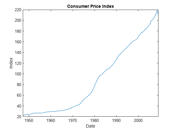
Plot the two series on separate plots.
figure; plot(DataTimeTable.Time,DataTimeTable.CPIAUCSL); title('Consumer Price Index') ylabel('Index') xlabel('Date')
figure; plot(DataTimeTable.Time,DataTimeTable.UNRATE); title('Unemployment Rate'); ylabel('Percent'); xlabel('Date');
Stabilize the CPI by converting it to a series of growth rates. Synchronize the two series by removing the first observation from the unemployment rate series.
rcpi = price2ret(DataTimeTable.CPIAUCSL); unrate = DataTimeTable.UNRATE(2:end);
Create a default VAR(4) model by using the shorthand syntax.
Mdl = varm(2,4)
Mdl = varm with properties: Description: "2-Dimensional VAR(4) Model" SeriesNames: "Y1" "Y2" NumSeries: 2 P: 4 Constant: [2×1 vector of NaNs] AR: {2×2 matrices of NaNs} at lags [1 2 3 ... and 1 more] Trend: [2×1 vector of zeros] Beta: [2×0 matrix] Covariance: [2×2 matrix of NaNs]
Mdl
is a varm
model object. All properties containing NaN
values correspond to parameters to be estimated given data.
Estimate the model using the entire data set.
EstMdl = estimate(Mdl,[rcpi unrate])
EstMdl = varm with properties: Description: "AR-Stationary 2-Dimensional VAR(4) Model" SeriesNames: "Y1" "Y2" NumSeries: 2 P: 4 Constant: [0.00171639 0.316255]' AR: {2×2 matrices} at lags [1 2 3 ... and 1 more] Trend: [2×1 vector of zeros] Beta: [2×0 matrix] Covariance: [2×2 matrix]
EstMdl
is an estimated varm
model object. It is fully specified because all parameters have known values. The description indicates that the autoregressive polynomial is stationary.
Display summary statistics from the estimation.
summarize(EstMdl)
AR-Stationary 2-Dimensional VAR(4) Model Effective Sample Size: 241 Number of Estimated Parameters: 18 LogLikelihood: 811.361 AIC: -1586.72 BIC: -1524 Value StandardError TStatistic PValue ___________ _____________ __________ __________ Constant(1) 0.0017164 0.0015988 1.0735 0.28303 Constant(2) 0.31626 0.091961 3.439 0.0005838 AR{1}(1,1) 0.30899 0.063356 4.877 1.0772e-06 AR{1}(2,1) -4.4834 3.6441 -1.2303 0.21857 AR{1}(1,2) -0.0031796 0.0011306 -2.8122 0.004921 AR{1}(2,2) 1.3433 0.065032 20.656 8.546e-95 AR{2}(1,1) 0.22433 0.069631 3.2217 0.0012741 AR{2}(2,1) 7.1896 4.005 1.7951 0.072631 AR{2}(1,2) 0.0012375 0.0018631 0.6642 0.50656 AR{2}(2,2) -0.26817 0.10716 -2.5025 0.012331 AR{3}(1,1) 0.35333 0.068287 5.1742 2.2887e-07 AR{3}(2,1) 1.487 3.9277 0.37858 0.705 AR{3}(1,2) 0.0028594 0.0018621 1.5355 0.12465 AR{3}(2,2) -0.22709 0.1071 -2.1202 0.033986 AR{4}(1,1) -0.047563 0.069026 -0.68906 0.49079 AR{4}(2,1) 8.6379 3.9702 2.1757 0.029579 AR{4}(1,2) -0.00096323 0.0011142 -0.86448 0.38733 AR{4}(2,2) 0.076725 0.064088 1.1972 0.23123 Innovations Covariance Matrix: 0.0000 -0.0002 -0.0002 0.1167 Innovations Correlation Matrix: 1.0000 -0.0925 -0.0925 1.0000
Forecast Responses from VAR(4) Model
This example follows from Fit VAR(4) Model to Matrix of Response Data.
Create and estimate a VAR(4) model for the CPI growth rate and unemployment rates. Treat the last ten periods as the forecast horizon.
load Data_USEconModel
cpi = DataTimeTable.CPIAUCSL;
unrate = DataTimeTable.UNRATE;
rcpi = price2ret(cpi);
unrate = unrate(2:end);
Y = [rcpi unrate];
Mdl = varm(2,4);
EstMdl = estimate(Mdl,Y(1:(end-10),:));
Forecast 10 responses using the estimated model and in-sample data as presample observations.
YF = forecast(EstMdl,10,Y(1:(end-10),:));
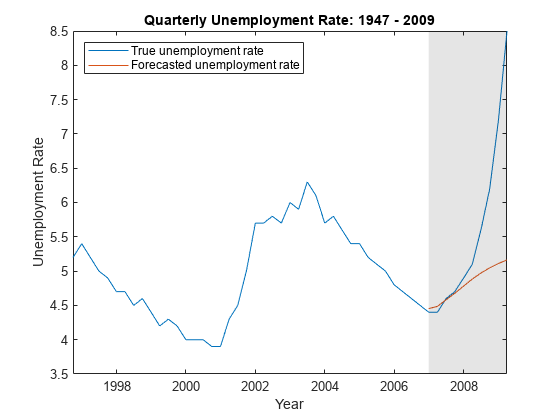
Plot the part of the series with their forecasted values on separate plots.
figure plot(DataTimeTable.Time(end - 50:end),rcpi(end - 50:end)); hold on plot(DataTimeTable.Time((end - 9):end),YF(:,1)) h = gca; fill(DataTimeTable.Time([end - 9 end end end - 9]),h.YLim([1,1,2,2]),'k',... 'FaceAlpha',0.1,'EdgeColor','none'); legend('True CPI growth rate','Forecasted CPI growth rate',... 'Location','NW') title('Quarterly CPI Growth Rate: 1947 - 2009') ylabel('CPI Growth Rate') xlabel('Year') hold off
figure plot(DataTimeTable.Time(end - 50:end),unrate(end - 50:end)); hold on plot(DataTimeTable.Time((end - 9):end),YF(:,2)) h = gca; fill(DataTimeTable.Time([end - 9 end end end - 9]),h.YLim([1,1,2,2]),'k',... 'FaceAlpha',0.1,'EdgeColor','none'); legend('True unemployment rate','Forecasted unemployment rate',... 'Location','NW') title('Quarterly Unemployment Rate: 1947 - 2009') ylabel('Unemployment Rate') xlabel('Year') hold off
More About
Vector Autoregression Model
A vector autoregression (VAR) model is a stationary multivariate time series model consisting of a system of m equations of m distinct response variables as linear functions of lagged responses and other terms.
A VAR(p) model in difference-equation notation and in reduced form is
yt is a
numseries
-by-1 vector of values corresponding tonumseries
response variables at time t, where t = 1,...,T. The structural coefficient is the identity matrix.c is a
numseries
-by-1 vector of constants.Φj is a
numseries
-by-numseries
matrix of autoregressive coefficients, where j = 1,...,p and Φp is not a matrix containing only zeros.xt is a
numpreds
-by-1 vector of values corresponding tonumpreds
exogenous predictor variables.β is a
numseries
-by-numpreds
matrix of regression coefficients.δ is a
numseries
-by-1 vector of linear time-trend values.εt is a
numseries
-by-1 vector of random Gaussian innovations, each with a mean of 0 and collectively anumseries
-by-numseries
covariance matrix Σ. For t ≠ s, εt and εs are independent.
Condensed and in lag operator notation, the system is
where , Φ(L)yt is
the multivariate autoregressive polynomial, and I is the
numseries
-by-numseries
identity matrix.
For example, a VAR(1) model containing two response series and three exogenous predictor variables has this form
Version History
Introduced in R2017aR2019b: Equality constraints on innovations covariance matrix
If you specify a positive definite innovations covariance matrix for the
Covariance
property, estimate
treats your
specification as an equality constraint in model estimation.
MATLAB 命令
您点击的链接对应于以下 MATLAB 命令:
请在 MATLAB 命令行窗口中直接输入以执行命令。Web 浏览器不支持 MATLAB 命令。
Select a Web Site
Choose a web site to get translated content where available and see local events and offers. Based on your location, we recommend that you select: .
You can also select a web site from the following list:
How to Get Best Site Performance
Select the China site (in Chinese or English) for best site performance. Other MathWorks country sites are not optimized for visits from your location.
Americas
- América Latina (Español)
- Canada (English)
- United States (English)
Europe
- Belgium (English)
- Denmark (English)
- Deutschland (Deutsch)
- España (Español)
- Finland (English)
- France (Français)
- Ireland (English)
- Italia (Italiano)
- Luxembourg (English)
- Netherlands (English)
- Norway (English)
- Österreich (Deutsch)
- Portugal (English)
- Sweden (English)
- Switzerland
- United Kingdom (English)