summarize

Display estimation results of vector autoregression (VAR) model

collapse all in page

Syntax

summarize(Mdl)

results = summarize(Mdl)

Description

summarize(Mdl) displays a summary of the VAR(p) model Mdl.

If Mdl is an estimated VAR model returned by estimate, then summarize prints estimation results to the MATLAB^® Command Window. The display includes a table of parameter estimates with corresponding standard errors, t statistics, and p-values. The summary also includes the loglikelihood, Akaike Information Criterion (AIC), and Bayesian Information Criterion (BIC) model fit statistics, as well as the estimated innovations covariance and correlation matrices.
If Mdl is an unestimated VAR model returned by varm, then summarize prints the standard object display (the same display that varm prints during model creation).

example

results = summarize(Mdl) returns one of the following variables and does not print to the Command Window.

If Mdl is an estimated VAR model, then results is a structure containing estimation results.
If Mdl is an unestimated VAR model, then results is a varm model object that is equal to Mdl.

example

Examples

collapse all

Fit VAR(4) Model to Matrix of Response Data

Open Live Script

Fit a VAR(4) model to the consumer price index (CPI) and unemployment rate series. Supply the response series as a numeric matrix.

Load the Data_USEconModel data set.

load Data_USEconModel

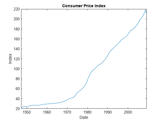
Plot the two series on separate plots.

figure;
plot(DataTimeTable.Time,DataTimeTable.CPIAUCSL);
title('Consumer Price Index')
ylabel('Index')
xlabel('Date')

Figure contains an axes object. The axes object with title Consumer Price Index, xlabel Date, ylabel Index contains an object of type line.

figure;
plot(DataTimeTable.Time,DataTimeTable.UNRATE);
title('Unemployment Rate');
ylabel('Percent');
xlabel('Date');

Figure contains an axes object. The axes object with title Unemployment Rate, xlabel Date, ylabel Percent contains an object of type line.

Stabilize the CPI by converting it to a series of growth rates. Synchronize the two series by removing the first observation from the unemployment rate series.

rcpi = price2ret(DataTimeTable.CPIAUCSL);
unrate = DataTimeTable.UNRATE(2:end);

Create a default VAR(4) model by using the shorthand syntax.

Mdl = varm(2,4)

Mdl = 
  varm with properties:

     Description: "2-Dimensional VAR(4) Model"
     SeriesNames: "Y1"  "Y2" 
       NumSeries: 2
               P: 4
        Constant: [2×1 vector of NaNs]
              AR: {2×2 matrices of NaNs} at lags [1 2 3 ... and 1 more]
           Trend: [2×1 vector of zeros]
            Beta: [2×0 matrix]
      Covariance: [2×2 matrix of NaNs]

Mdl is a varm model object. All properties containing NaN values correspond to parameters to be estimated given data.

Estimate the model using the entire data set.

EstMdl = estimate(Mdl,[rcpi unrate])

EstMdl = 
  varm with properties:

     Description: "AR-Stationary 2-Dimensional VAR(4) Model"
     SeriesNames: "Y1"  "Y2" 
       NumSeries: 2
               P: 4
        Constant: [0.00171639 0.316255]'
              AR: {2×2 matrices} at lags [1 2 3 ... and 1 more]
           Trend: [2×1 vector of zeros]
            Beta: [2×0 matrix]
      Covariance: [2×2 matrix]

EstMdl is an estimated varm model object. It is fully specified because all parameters have known values. The description indicates that the autoregressive polynomial is stationary.

Display summary statistics from the estimation.

summarize(EstMdl)

 
   AR-Stationary 2-Dimensional VAR(4) Model
 
    Effective Sample Size: 241
    Number of Estimated Parameters: 18
    LogLikelihood: 811.361
    AIC: -1586.72
    BIC: -1524
 
                      Value       StandardError    TStatistic      PValue  
                   ___________    _____________    __________    __________

    Constant(1)      0.0017164      0.0015988         1.0735        0.28303
    Constant(2)        0.31626       0.091961          3.439      0.0005838
    AR{1}(1,1)         0.30899       0.063356          4.877     1.0772e-06
    AR{1}(2,1)         -4.4834         3.6441        -1.2303        0.21857
    AR{1}(1,2)      -0.0031796      0.0011306        -2.8122       0.004921
    AR{1}(2,2)          1.3433       0.065032         20.656      8.546e-95
    AR{2}(1,1)         0.22433       0.069631         3.2217      0.0012741
    AR{2}(2,1)          7.1896          4.005         1.7951       0.072631
    AR{2}(1,2)       0.0012375      0.0018631         0.6642        0.50656
    AR{2}(2,2)        -0.26817        0.10716        -2.5025       0.012331
    AR{3}(1,1)         0.35333       0.068287         5.1742     2.2887e-07
    AR{3}(2,1)           1.487         3.9277        0.37858          0.705
    AR{3}(1,2)       0.0028594      0.0018621         1.5355        0.12465
    AR{3}(2,2)        -0.22709         0.1071        -2.1202       0.033986
    AR{4}(1,1)       -0.047563       0.069026       -0.68906        0.49079
    AR{4}(2,1)          8.6379         3.9702         2.1757       0.029579
    AR{4}(1,2)     -0.00096323      0.0011142       -0.86448        0.38733
    AR{4}(2,2)        0.076725       0.064088         1.1972        0.23123

 
   Innovations Covariance Matrix:
    0.0000   -0.0002
   -0.0002    0.1167

 
   Innovations Correlation Matrix:
    1.0000   -0.0925
   -0.0925    1.0000

Compare Several VAR Model Fits

Open Live Script

Consider these four VAR models of consumer price index (CPI) and unemployment rate: VAR(0), VAR(1), VAR(4), and VAR(8). Using historical data, estimate each, and then compare the model fits using the resulting BIC.

Load the Data_USEconModel data set. Declare variables for the consumer price index (CPI) and unemployment rate (UNRATE) series. Remove any missing values from the beginning of the series.

load Data_USEconModel
cpi = DataTimeTable.CPIAUCSL;
unrate = DataTimeTable.UNRATE;
idx = all(~isnan([cpi unrate]),2);
cpi = cpi(idx);
unrate = unrate(idx);

Stabilize CPI by converting it to a series of growth rates. Synchronize the two series by removing the first observation from the unemployment rate series.

rcpi = price2ret(cpi);
unrate = unrate(2:end);

Within a loop:

Create a VAR model using the shorthand syntax.
Estimate the VAR Model. Reserve the maximum value of p as presample observations.
Store the estimation results.

numseries = 2;
p = [0 1 4 8];
estMdlResults = cell(numel(p),1); % Preallocation
Y0 = [rcpi(1:max(p)) unrate(1:max(p))];
Y = [rcpi((max(p) + 1):end) unrate((max(p) + 1):end)];

for j = 1:numel(p)
    Mdl = varm(numseries,p(j));
    EstMdl = estimate(Mdl,Y,'Y0',Y);
    estMdlResults{j} = summarize(EstMdl);
end

estMdlResults is a 4-by-1 cell array of structure arrays containing the estimation results of each model.

Extract the BIC from each set of results.

BIC = cellfun(@(x)x.BIC,estMdlResults)

BIC = 4×1
10³ ×

   -0.7153
   -1.3678
   -1.4378
   -1.3853

The model corresponding to the lowest BIC has the best fit among the models considered. Therefore, the VAR(4) is the best fitting model.

Input Arguments

collapse all

`Mdl` — VAR model
`varm` model object

VAR model, specified as a varm model object returned by estimate, varm, or varm (a vecm function).

Output Arguments

collapse all

`results` — Model summary
structure array | `varm` model object

Model summary, returned as a structure array or a varm model object.

If Mdl is an estimated VAR model, then results is a structure array containing the fields in this table.

Field	Description
`Description`	Model summary description (string)
`SampleSize`	Effective sample size (numeric scalar)
`NumEstimatedParameters`	Number of estimated parameters (numeric scalar)
`LogLikelihood`	Optimized loglikelihood value (numeric scalar)
`AIC`	Akaike information criterion (numeric scalar)
`BIC`	Bayesian information criterion (numeric scalar)
`Table`	Parameter estimates with corresponding standard errors, t statistics (estimate divided by standard error), and p-values (assuming normality); a table with rows corresponding to model parameters
`Covariance`	Estimated residual covariance matrix (the maximum likelihood estimate), a `Mdl.NumSeries`-by-`Mdl.NumSeries` numeric matrix with rows and columns corresponding to the innovations in the response equations ordered by the data `Y`
`Correlation`	Estimated residual correlation matrix, its dimensions correspond to the dimensions of `Covariance`

summarize uses mvregress to implement multivariate normal, maximum likelihood estimation. For more details on estimates and standard errors, see Estimation of Multivariate Regression Models.

If Mdl is an unestimated VAR model, then results is a varm model object that is equal to Mdl.

Version History

Introduced in R2017a

summarize

Syntax

Description

Examples

Fit VAR(4) Model to Matrix of Response Data

Compare Several VAR Model Fits

Input Arguments

`Mdl` — VAR model
`varm` model object

Output Arguments

`results` — Model summary
structure array | `varm` model object

Version History

See Also

Objects

Functions

Topics

summarize

Syntax

Description

Examples

Fit VAR(4) Model to Matrix of Response Data

Compare Several VAR Model Fits

Input Arguments

Mdl — VAR model varm model object

Output Arguments

results — Model summary structure array | varm model object

Version History

See Also

Objects

Functions

Topics

`Mdl` — VAR model
`varm` model object

`results` — Model summary
structure array | `varm` model object