Forecast Multivariate Model Responses Using Econometric Modeler App
This example shows how to estimate a VAR model, and then generate forecasts from the model by using the Econometric Modeler app. This example follows from the analysis in Compare Predictive Performance After Creating Models Using Econometric Modeler.
Although the example uses a VAR model, the workflow is similar for all multivariate models available in Econometric Modeler, such as VEC models. Econometric Modeler cannot forecast models containing an exogenous predictor variables, such as VARX models.
The data set, which is stored in Data_USEconModel.mat, contains
the raw, quarterly US GDP, M1 money supply, and 3-month T-bill rate, among other
series, from 1947 through 2009.
Load and Import Data into Econometric Modeler
At the command line, load the Data_USEconModel.mat data
set.
load Data_USEconModelAt the command line, open the Econometric Modeler app.
econometricModeler
Alternatively, open the app from the apps gallery (see Econometric Modeler).
Import DataTimeTable into the app:
On the Modeler tab, in the Import section, click the Import button
 .
.In the Import Data dialog box, select the check box for the
DataTimeTablevariable.Click Import.
GDP, M1SL, and
TB3MS, among other series, appear in the
Time Series pane, and a time series plot containing all
series appears in the figure window.
Transform Series
Remove the exponential trend from the GDP and M1 money supply series by
applying the log transform to each series. Click the
Modeler tab, and then, in the Time
Series pane, click GDP and
Ctrl click M1SL. In the
Transforms section, click Log.
The transformed series GDP_Log and
M1SL_Log appear in the Time
Series pane, and their time series plot appears in the
Plot(GDP_Log) figure window.
Stabilize the series by applying the first difference to each series.
Click the Modeler tab, and then, in the Time Series pane, click
GDP_Logand Ctrl+clickM1SL_LogandTB3MS.In the Transforms section, click Difference. The transformed series
GDP_Log_Diff,M1SL_Log_Diff, andTB3MS_Diffappear in the Time Series pane, and their time series plot appears in the Plot(GDP_Log_Diff) figure window.Rename
GDP_Log_DiffandM1SL_Log_DifftoGDPRateandM1SLRateby clicking their names twice in the Time Series pane, and typing their new names.
Estimate VAR Models
Fit a 3-D VAR(2) model to the US quarterly GDP growth rate series
GDPRate, M1 money supply growth rate series
M1SLRate, and change in the 3-month treasury bill
rate series TB3MS_Diff.
In the Time Series pane, click
GDPRateand Ctrl+clickM1SLRateandTB3MS_Diff.In the Models section, click VAR.
In the VAR Model Parameters dialog box, set Autoregressive Order (p) to
2. Then, click Estimate.The model variable
VARappears in the Models pane, its value appears in the Preview pane, and its estimation summary appears in the Fit(VAR) document.
Forecast Estimated Model
Forecast the model into a 10-year (40-period) horizon.
In the Models pane, select the
VARmodel.On the Modeler tab, in the Forecast section, click Forecast.
In the Forecast Model Response dialog box, set Number of periods in forecast horizon to
40. Click Forecast.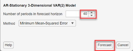
In the Forecasts pane, a variable
For_VAR appears. This variable is a structure
array with the following fields:
Forecast— fh-by-m matrix of forecasted responses, with rows corresponding to the fh specified periods in the forecast horizon and columns corresponding to the variables in the model.UpperConfidenceBound— fh-by-m matrix of upper confidence bounds of the pointwise 95% Wald-based forecast intervalsLowerConfidenceBound— fh-by-m matrix of lower confidence bounds of the pointwise 95% Wald-based forecast intervals
Note
In the Forecast Model Response dialog box, when you set
Method to
Simulation, Econometric Modeler computes and
returns Monte Carlo simulation statistics:
Forecast— fh-by-m matrix of pointwise means of the forecasted pathsUpperConfidenceBound— fh-by-1matrix of upper confidence bounds of the pointwise 95% percentile-based forecast intervalsLowerConfidenceBound— fh-by-1matrix of lower confidence bounds of the pointwise 95% percentile-based forecast intervals
In the right pane, in the For(VAR) tab, is a plot
containing the following time series associated with the
GDPRate variable:
The time series data (blue line)
Forecasts (dashed blue line)
The pointwise 95% percentile-based confidence intervals (light blue region)
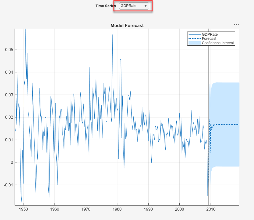
In the long run, the rate settles at around 1.5% on average, but expected to be within the bounds of slightly below 0% to 3.5%.
Plot the TB3MS_Diff forecasts and forecast
intervals. In the right pane, in the For(VAR) window, click
Time Series >
TB3MS_Diff.
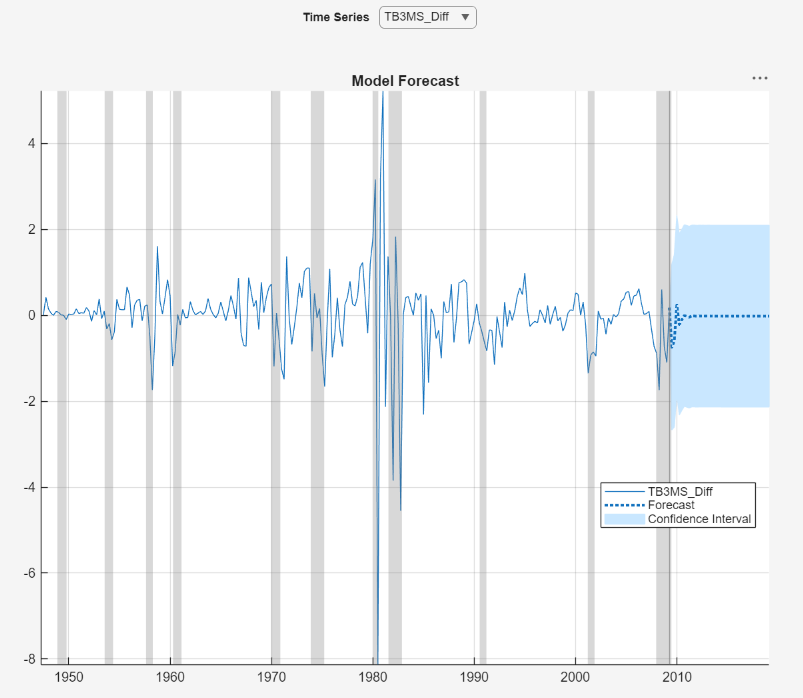
In the long run, the change in the 3-month treasury bill settles slightly below 0, and is expected to be in the bounds of -2 to 2.