Analyze US Unemployment Rate Using Threshold-Switching Model

Open Live Script

Asymmetry of the business cycle is a factor in many econometric models. In general, periods of contraction occur more quickly than periods of expansion, and changes in level can be persistent. The unemployment rate is a common indicator of the cycle.

This example shows how to describe the dynamics of the monthly US unemployment rate using a threshold-switching dynamic regression model. Specifically, the example follows an analysis in [2]:

Determine an adequate autoregressive (AR) lag order by fitting nested AR models to the data and then by comparing information criteria of the estimated models.
Fit a self-exciting, logistic-transition, smooth, threshold-switching autoregressive (LSTAR) model containing AR submodels of the order determined in step 1.
Evaluate LSTAR model states relative to empirical periods of contraction and expansion.
Compare forecasts generated by the estimated AR and LSTAR models.

Load and Preprocess Data

Load the monthly data for the US unemployment rate during the 45-year period 1954−1998.

load Data_Unemployment

The unemployment rate series Data is a 45-by-12 matrix of measurements, with rows corresponding to successive years and columns corresponding to successive months.

Orient the data so that the series is a vector of consecutive measurements.

Data = Data';
UN = Data(:);

Create a datetime vector of observation dates. Store the data in a timetable.

numYears = numel(dates);
numMonths = 12*numYears - 1;
t = datetime(dates(1),1,1) + calmonths((0:numMonths)');
DTT = timetable(UN,RowTimes=t);

Plot the series and overlay recession bands, reported by the National Bureau of Economic Research.

figure
plot(t,UN)
recessionplot
ylabel("Rate (%)")
title("Monthly US Unemployment Rate, 1954−1998")

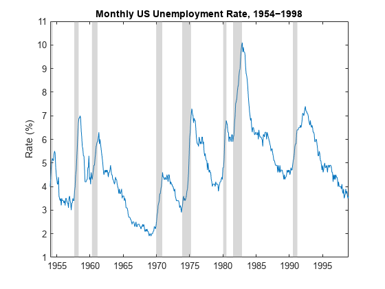
Figure contains an axes object. The axes object with title Monthly US Unemployment Rate, 1954−1998, ylabel Rate (%) contains 9 objects of type line, patch.

Asymmetric periods of economic contraction (upward swings in unemployment) and expansion (gradual declines) are evident. Expansions following the recession in the early 1970s fail to return to previous levels.

To compare models, partition the data into an initial subsample of the first 35 years, for model estimation, and a holdout sample of the remaining 10 years, for evaluating forecast performance.

startHO = t(1) + calyears(35);
UNEst = UN(t < startHO);    % First 35 years
UNFor = UN(t >= startHO);   % Final 10 years

Determine Autoregressive Order for Submodels

To determine an appropriate autoregressive order for submodels of the threshold-switching model, fit standard autoregressive models with lags from 1 through 10 to the estimation sample. To compare the in-sample fits among the estimated models, compute the Akaike information criterion (AIC) for each model.

AIC = zeros(10,1);  % Preallocation
maxLag = 10;

for p = 1:maxLag
    MdlAR = arima(p,0,0);   % Model template for estimation
    [~,~,logL] = estimate(MdlAR,UNEst,Display="off");
    AIC(p) = aicbic(logL,p+1);    
end

figure
plot(AIC,"o-")
xlabel("AR Order (p)")
ylabel("AIC")
title("AR(p) Model AIC")

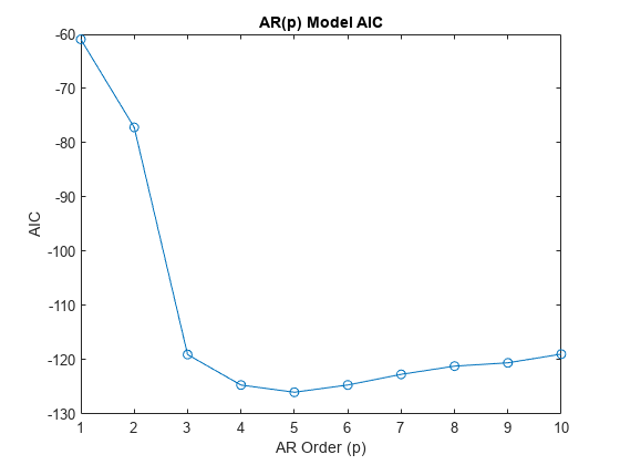
Figure contains an axes object. The axes object with title AR(p) Model AIC, xlabel AR Order (p), ylabel AIC contains an object of type line.

The plot indicates an AR order of 5 minimizes the AIC for the data.

Fit an AR(5) model to the data.

MdlAR5 = arima(5,0,0);
EstMdlAR5 = estimate(MdlAR5,UNEst);

 
    ARIMA(5,0,0) Model (Gaussian Distribution):
 
                  Value      StandardError    TStatistic      PValue   
                _________    _____________    __________    ___________

    Constant     0.082534       0.038097         2.1664        0.030278
    AR{1}          1.0794       0.046648          23.14     1.8452e-118
    AR{2}         0.17947       0.083388         2.1523        0.031377
    AR{3}        -0.14845       0.071375        -2.0799        0.037537
    AR{4}       -0.038119       0.064947       -0.58693         0.55725
    AR{5}       -0.089782       0.052936        -1.6961        0.089875
    Variance     0.042155      0.0021407         19.693      2.4939e-86

Fit Threshold-Switching Model to Data

For comparison, create a logistic-transition, smooth, threshold-switching autoregressive model with AR(5) submodels.

The unemployment rate exhibits considerable short-term fluctuations. The analysis in [2], using a decision rule in [1], suggests the trailing 12-month change in the lagged unemployment rate $Δ_{12}$ UN(t-1) as a more indicative self-exciting threshold variable. Follow this procedure:

Create a timetable such that the first column contains the raw series, the second column contains the first lag of series, and the third column contains the 13th lag by using the lagmatrix function.
For each observation, create the threshold variable by subtracting the 13th lag from the first lag.
Remove any trailing missing values from the resulting timetable.
Create estimation and validation data sets.

DTTLags = lagmatrix(DTT,[0 1 13]);
DTTLags.Z = DTTLags.Lag1UN - DTTLags.Lag13UN; % Threshold variable data
DTTLags = rmmissing(DTTLags);
DTTLags = renamevars(DTTLags,"Lag0UN","UN");  
DTTEst = DTTLags(DTTLags.Time < startHO,:);   % Estimation data
DTTFor = DTTLags(DTTLags.Time >= startHO,:);  % Validation data

Create a model template that specifies all parameters in an unconstrained LSTAR model are estimable. To initialize the parameter searc, create a fully specified logistic threshold transition with a transition mid-level at 0 and transition rate of 5.

tt = threshold(NaN,Rates=NaN,Type="logistic");
mdl = arima(5,0,0);
MdlLSTAR5 = tsVAR(tt,[mdl mdl],Covariance=NaN);

tt0 = threshold(0,Rates=5,Type="logistic");

Estimate the unconstrained LSTAR model. Specify that the threshold variable is exogenous and supply its data. Visually track the loglikelihood during the estimation procedure. Restrict the search domain of the transition rate to a maximum of 50.

figure
[EstMdlLSTAR5,EstSE] = estimate(MdlLSTAR5,tt0,DTTEst.UN, ...
    Type="exogenous",Z=DTTEst.Z,MaxRate=50,IterationPlot=true);

Figure contains an axes object. The axes object with title Threshold Search Algorithm, xlabel Iteration, ylabel Log-Likelihood contains an object of type line.

The loglikelihood converges in less than 10 iterations.

Analyze Estimated LSTAR Model

Display the estimated threshold transition.

ttEst = EstMdlLSTAR5.Switch

ttEst = 
  threshold with properties:

          Type: 'logistic'
        Levels: 0.1154
         Rates: 8.5253
    StateNames: ["1"    "2"]
     NumStates: 2

The estimated threshold level is near 0, indicating that the model distinguishes submodels representing negative and positive 12-month changes in unemployment.

Evaluate the transition function by using ttdata to plot values of the transition function over the estimation period.

TFData = ttdata(ttEst,DTTEst.Z);

figure
plot(DTTEst.Time,TFData)
recessionplot
title("Transition Function vs. Time")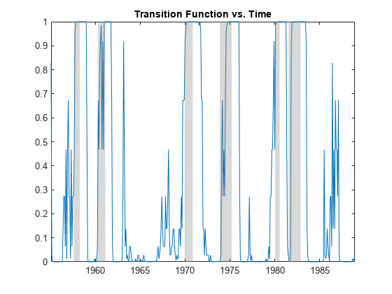

Figure contains an axes object. The axes object with title Transition Function vs. Time contains 7 objects of type line, patch.

figure
plot(DTTEst.Z,TFData,"o")
xlabel("Z = \Delta_{12}UN_{{\it t}-1}")
title("Transition Function vs. Threshold Variable")

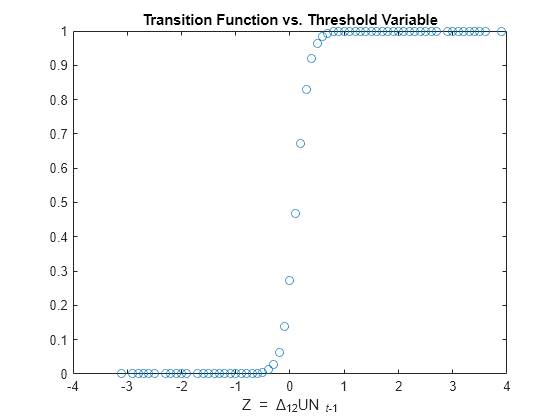
Figure contains an axes object. The axes object with title Transition Function vs. Threshold Variable, xlabel Z = blank Delta indexOf 12 baseline UN indexOf blank t - 1 baseline contains a line object which displays its values using only markers.

Plots of the transition function data show the threshold variable sampling both the expansion and contraction regimes, with switching triggered by recessions.

Compare the estimated AR(5) submodels. Negative unemployment rates indicate an expansion (regime 1) and positive rates indicate a contraction (regime 2).

ExpansionRegime = EstMdlLSTAR5.Submodels(1)

ExpansionRegime = 
  varm with properties:

     Description: "AR-Stationary 1-Dimensional VAR(5) Model"
     SeriesNames: "Y1" 
       NumSeries: 1
               P: 5
        Constant: 0.0565741
              AR: {0.744782 0.327556 -0.075966 ... and 2 more} at lags [1 2 3 ... and 2 more]
           Trend: 0
            Beta: [1×0 matrix]
      Covariance: NaN

ExpansionRegime.AR

ans=1×5 cell array
    {[0.7448]}    {[0.3276]}    {[-0.0760]}    {[0.0696]}    {[-0.0870]}

ContractionRegime = EstMdlLSTAR5.Submodels(2)

ContractionRegime = 
  varm with properties:

     Description: "AR-Stationary 1-Dimensional VAR(5) Model"
     SeriesNames: "Y1" 
       NumSeries: 1
               P: 5
        Constant: 0.148029
              AR: {1.30079 0.00307393 -0.183726 ... and 2 more} at lags [1 2 3 ... and 2 more]
           Trend: 0
            Beta: [1×0 matrix]
      Covariance: NaN

ContractionRegime.AR

ans=1×5 cell array
    {[1.3008]}    {[0.0031]}    {[-0.1837]}    {[-0.2045]}    {[0.0574]}

The AR(5) submodels in the expansion and contraction regimes have distinct lag structures.

Compare Forecast Performance of Models

Visually compare the forecast performance of the AR(5) and LSTAR models.

Forecast AR(5) Model

Use the forecast object function of the arima object to compute the long-term, minimum mean square error (MMSE) forecast of the AR(5) model of the data, 120 months into the forecast horizon.

fh = height(DTTFor);
[UNF,MSE] = forecast(EstMdlAR5,fh,DTTEst.UN);

figure
plot(DTTFor.Time,UNF,"r")
mu = EstMdlAR5.UnconditionalMean;
yline(mu,'k--')
h = gca;
ylim([h.YLim(1),mu + 0.01])

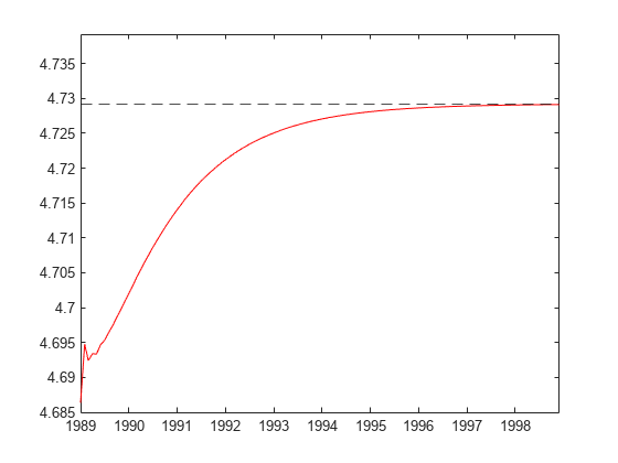
Figure contains an axes object. The axes object contains 2 objects of type line, constantline.

After 5 months of short-term adjustment as lagged terms from UNEst are sampled, the forecast approaches the unconditional mean of the model.

Use the supporting function plotforecasts to plot the forecasts and approximate 95% forecast intervals at the scale of the original data.

plotforecasts(DTTEst,DTTFor,UNF,MSE,"AR Forecast")

Figure contains an axes object. The axes object with title AR Forecast contains 6 objects of type line, patch. These objects represent Interval, Actual, Optimal.

The point forecast fails to capture the cyclical component in the data and the interval forecast fails to distinguish among a wide range of forecast paths.

Forecast LSTAR Model

Forecasting a self-exciting threshold-switching model poses a challenge. To compute a long-term forecast threshold variable data ( $z_{t}$ ) in the forecast period is required. However, threshold variable data in the forecast period depends on the forecast itself. How the threshold variable data is introduced depends on the context. This example considers two settings:

Analysis of historical data, in which holdout data is available in the forecast period.
Real-time analysis, in which forecast data is generated iteratively.

Model Predictive Performance Using Historical Data

This example shows the following two scenarios for forecasting when threshold data is available in the forecast period:

The entire holdout sample of proxy data is introduced at the start of the forecast.
Holdout data is introduced "just in time" in iterative, one-step-ahead forecasts.

Supply the entire holdout sample as a proxy for data that is normally available iteratively in the forecast period. Plot optimal and Monte Carlo forecasts.

rng(0) % For reproducibility of Monte Carlo forecasts

UNF1 = forecast(EstMdlLSTAR5,DTTEst.UN,fh,Type="exogenous", ...
    Z=DTTFor.Z); % Optimal
[UNF2,EstVar] = forecast(EstMdlLSTAR5,DTTEst.UN,fh,Type="exogenous", ...
    Z=DTTFor.Z); % Monte Carlo forecasts and forecast standard errors 

plotforecasts(DTTEst,DTTFor,[UNF1 UNF2],EstVar,"LSTAR Forecasts: Proxy Data")

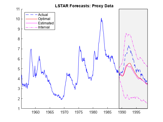
Figure contains an axes object. The axes object with title LSTAR Forecasts: Proxy Data contains 7 objects of type line, patch. These objects represent Interval, Actual, Optimal, Estimated.

The LSTAR forecasts are more successful than the AR(5) forecasts at capturing the cyclical component in the data.

Supply the holdout sample iteratively to compute a series of one-step-ahead forecasts. Plot the optimal and Monte Carlo forecasts.

UNEstIter = UNEst;

for i = 1:fh
    Zi = UNEstIter(end)-UNEstIter(end-12);
    UNF1(i) = forecast(EstMdlLSTAR5,UNEstIter,1,Type="exogenous", ...
        Z=Zi);  % Optimal
    [UNF2(i),EstVar] = forecast(EstMdlLSTAR5,UNEstIter,1, ...
        Type="exogenous",Z= Zi);    % Estimated
    UNEstIter = [UNEstIter; UNFor(i)];  %#ok Update UNEstIter with UNFor
end

plotforecasts(DTTEst,DTTFor,[UNF1 UNF2],EstVar, ...
    "LSTAR Forecasts: Just-in-Time Threshold Data")

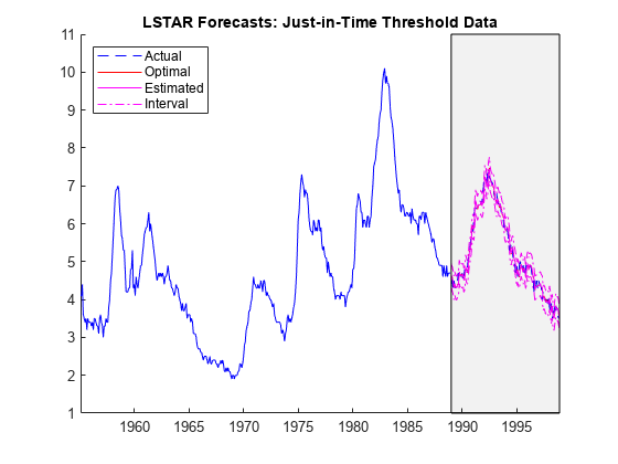
Figure contains an axes object. The axes object with title LSTAR Forecasts: Just-in-Time Threshold Data contains 7 objects of type line, patch. These objects represent Interval, Actual, Optimal, Estimated.

The forecasts closely track the holdout sample, as corrections become available at each time step.

Model Predictive Performance in Real Time

In practice, self-exciting threshold variable data becomes available only iteratively, suggesting a rolling series of short-term forecasts. This example shows the following two scenarios for forecasting the LSTAR model in the absence of holdout data:

Iteratively form the threshold variable $z_{t}$ using optimal one-step-ahead forecasts.
Iteratively form the threshold variable $z_{t}$ using Monte Carlo one-step-ahead forecasts.

Implement a rolling one-step-ahead optimal forecast. Plot the forecasts and corresponding approximate 95% forecast intervals.

UNF1 = zeros(fh,1); % Preallocate forecast arrays
UNF2 = zeros(fh,1);
UNEstIter = DTTEst.UN;

for i = 1:120
    Zi = UNEstIter(end) - UNEstIter(end-12);
    UNF1(i) = forecast(EstMdlLSTAR5,UNEstIter,1,Type="exogenous", ...
        Z=Zi); % Optimal one-step-ahead forecast
    [UNF2(i),EstVar] = forecast(EstMdlLSTAR5,UNEstIter,1, ...
        Type="exogenous",Z=Zi); % Monte Carlo one-step-ahead forecast
    UNEstIter = [UNEstIter; UNF1(i)];   %#ok Update UNEstIter with UNF1
end

plotforecasts(DTTEst,DTTFor,[UNF1 UNF2],EstVar, ...
    "LSTAR Forecasts: Optimal Forecast Threshold Data")

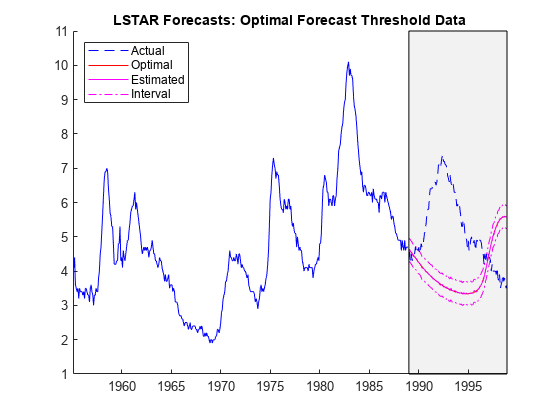
Figure contains an axes object. The axes object with title LSTAR Forecasts: Optimal Forecast Threshold Data contains 7 objects of type line, patch. These objects represent Interval, Actual, Optimal, Estimated.

The forecast does not track the holdout sample, but it captures essential statistical dynamics in the estimation sample, including the approximate shape and period of the cycle. This is one of the main benefits of using a switching model.

Implement a rolling one-step-ahead Monte Carlo forecast. Plot the forecasts and corresponding approximate 95% forecast intervals.

UNEstIter = UNEst;  % Reset UNEstIter

for i = 1:fh
    Zi = UNEstIter(end) - UNEstIter(end-12);
    UNF1(i) = forecast(EstMdlLSTAR5,UNEstIter,1,Type="exogenous", ...
        Z=Zi);
    [UNF2(i),EstVar] = forecast(EstMdlLSTAR5,UNEstIter,1, ...
        Type="exogenous",Z=Zi);
    UNEstIter = [UNEstIter; UNF2(i)]; %#ok Update UNEstIter with UNF2
end

plotforecasts(DTTEst,DTTFor,[UNF1 UNF2],EstVar, ...
    "LSTAR Forecasts: Estimated Forecast Threshold Data")

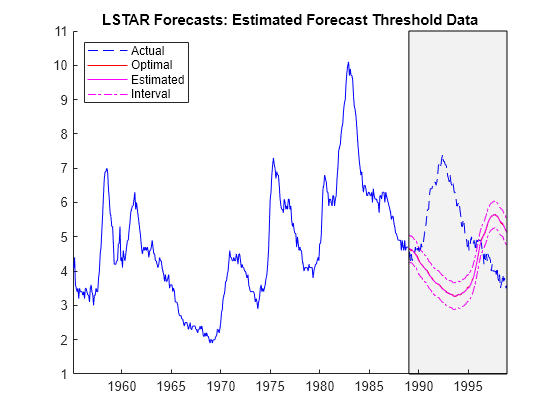
Figure contains an axes object. The axes object with title LSTAR Forecasts: Estimated Forecast Threshold Data contains 7 objects of type line, patch. These objects represent Interval, Actual, Optimal, Estimated.

The dynamic behavior of these forecasts is similar to the behavior of the optimal forecasts.

Supporting Function

The plotforecasts supporting function plots the data and the forecast with the 95% forecast intervals.

function plotforecasts(DTTEst,DTTFor,UNF,MSE,tlt)
    % Inputs:    
    % DTTEst: Timetable of data in the estimation sample
    % DTTFor: Timetable of data in the forecast sample
    % UNF: Matrix of optimal and, optionally, estimated forecasts
    % MSE: Vector of corresponding forecast MSEs
    % tlt: String containing the plot title

    numforecasts = size(UNF,2);
    lbls = ["Actual" "Optimal" "Interval"];

    figure
    hold on
    plot(DTTEst.Time,DTTEst.UN,"b");
    h(numforecasts + 2) = plot(DTTFor.Time,UNF(:,end)+1.96*sqrt(MSE),"m-.");    % Upper 95% confidence level
    plot(DTTFor.Time,UNF(:,end)-1.96*sqrt(MSE),"m-.");                          % Lower 95% confidence level
    h(1) = plot(DTTFor.Time,DTTFor.UN,"b--");
    h(2) = plot(DTTFor.Time,UNF(:,1),"r");
    if(numforecasts == 2)
        h(3) = plot(DTTFor.Time,UNF(:,2),"m");
        lbls = [lbls(1:2) "Estimated" lbls(end)];
    end
    yfill = [ylim fliplr(ylim)];
    xfill = DTTFor.Time([1 1 end end]);
    fill(xfill,yfill,"k",FaceAlpha=0.05);
    legend(h,lbls,Location="northwest")
    title(tlt)
    hold off
end

References

[1] Teräsvirta, Tima. "Modelling Economic Relationships with Smooth Transition Regressions." In A. Ullahand and D.E.A. Giles (eds.), Handbook of Applied Economic Statistics, 507–552. New York: Marcel Dekker, 1998.

[2] van Dijk, Dick. Smooth Transition Models: Extensions and Outlier Robust Inference. Rotterdam, Netherlands: Tinbergen Institute Research Series, 1999.