Main Content

impulse

Generate regression model with ARIMA errors impulse response function (IRF)

Description

y = impulse(Mdl) returns the impulse response function (IRF) of the input regression model with ARIMA time series errors. impulse returns the dynamic responses starting at period 0, during which impulse applies a unit shock to the innovation.

example

y = impulse(Mdl,numObs) returns the numObs dynamic responses from periods 0 through numObs – 1.

example

impulse(___) plots a discrete stem plot of the IRF of the input regression model with ARIMA errors to the current axes, using any of the input argument combinations in the previous syntaxes.

example

impulse(ax,___) plots on the axes specified by ax instead of the current axes (gca). ax can precede any of the input argument combinations in the previous syntaxes. (since R2024a)

[___,h] = impulse(___) plots the IRF and additionally returns handles to the plotted graphics objects. Use elements of h to modify properties of the plot after you create it. (since R2024a)

Examples

collapse all

Specify the following regression model with ARMA(2,1) errors:

yt=Xt[0.1-0.2]+utut=0.5ut-1-0.8ut-2+εt-0.5εt-1,

where εt is Gaussian with variance 0.1.

Mdl = regARIMA(Intercept=0,AR={0.5 -0.8},MA=-0.5, ...
    Beta=[0.1; -0.2],Variance=0.1);

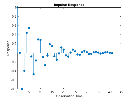
Time the calculation of and plot the impulse response function without specifying the number of observations.

impulse(Mdl)

Figure contains an axes object. The axes object with title Impulse Response, xlabel Observation Time, ylabel Response contains an object of type stem.

The model is stationary; the impulse response function decays in a sinusoidal pattern.

Specify the following regression model with ARMA(2,1) errors:

yt=Xt[0.1-0.2]+utut=0.5ut-1-0.8ut-2+εt-0.5εt-1,

where εt is Gaussian with variance 0.1.

Mdl = regARIMA(Intercept=0,AR={0.5 -0.8},MA=-0.5, ...
    Beta=[0.1; -0.2],Variance=0.1);

Store the impulse response function for 15 periods.

y = impulse(Mdl,15)
y = 15×1

    1.0000
         0
   -0.8000
   -0.4000
    0.4400
    0.5400
   -0.0820
   -0.4730
   -0.1709
    0.2930
      ⋮

The length of the output impulse response series is numObs. y(1) is the IRF at period 0, during which impulse shocks Mdl. y(15) is the IRF at period 14.

Input Arguments

collapse all

Fully specified regression model with ARIMA errors, specified as a regARIMA model object created by regARIMA or estimate.

The properties of Mdl cannot contain NaN values.

Number of periods to include in the IRF (the number of periods for which impulse computes the IRF), specified as a positive integer.

If you specify numObs, impulse computes the IRF by filtering a unit impulse, followed by a vector of zeros of length numObs – 1, through the model Mdl. In this case, the filtering algorithm is efficient.

By default, impulse determines the number of periods in the IRF by using the polynomial division algorithm of the underlying lag operator polynomials. For more details, see Algorithms.

Example: impulse(Mdl,10) returns the IRF for 10 periods.

Data Types: double

Since R2024a

Axes on which to plot, specified as an Axes object.

By default, impulse plots to the current axes (gca).

Output Arguments

collapse all

IRF, returned as a numeric column vector. If you specify numObs, Y has length numObs. If you do not specify numObs, the tolerances of the underlying lag operator polynomial division algorithm determine the length of y.

y(j) is the impulse response of yt at period j – 1. y(0) represents the impulse response during the period in which impulse applies the unit shock to the innovation (ε0 = 1).

Since R2024a

Handles to plotted graphics objects, returned as a graphics array. h contains unique plot identifiers, which you can use to query or modify properties of the plot.

More About

collapse all

Impulse Response Function

The impulse response function for regression models with ARIMA errors is the dynamic response of the system to a single impulse, or innovation shock, of unit size. The specific impulse response calculated by impulse is the dynamic multiplier, defined as the partial derivative of the output response with respect to an innovation shock at time 0.

For a regression model with ARIMA errors, yt, unconditional disturbances ut, and innovation series εt, the impulse response at time j, Ψj, is given by

ψj=yjε0=ujε0.

Expressed as a function of time, the sequence of dynamic multipliers, Ψ1, Ψ2,..., measures the sensitivity of the process to a purely transitory change in the innovation process. impulse computes the impulse response function by shocking the system with a unit impulse ε0 = 1, with all past observations of yt and all future shocks of εt set to 0. The impulse response function is the partial derivative of the ARIMA process with respect to an innovation shock at time 0. Because of this, the presence of an intercept or a regression component corresponding to predictors in the model has no effect on the output.

This impulse response is sometimes called the forecast error impulse response, because the innovations, εt, can be interpreted as the one-step-ahead forecast errors.

Tips

  • To improve performance of the filtering algorithm, specify the number of observations, numObs, to include in the impulse response.

Algorithms

  • If you specify the number of periods numObs, impulse computes the IRF by filtering a unit shock followed by an appropriate length vector of zeros. The filtering algorithm is very fast and results in an IRF of numObs length.

  • If you do not specify numObs, impulse implements this procedure:

    1. Convert the error model to a pure moving average (MA) polynomial by using the relatively slow lag operator polynomial division algorithm.

    2. Truncate the pure MA polynomial according to default tolerances because the polynomial is generally of infinite degree.

    This procedure produces an IRF of generally unknown length. For more details, see LagOp and mldivide.

References

[1] Box, George E. P., Gwilym M. Jenkins, and Gregory C. Reinsel. Time Series Analysis: Forecasting and Control. 3rd ed. Englewood Cliffs, NJ: Prentice Hall, 1994.

[2] Enders, Walter. Applied Econometric Time Series. Hoboken, NJ: John Wiley & Sons, Inc., 1995.

[3] Hamilton, James D. Time Series Analysis. Princeton, NJ: Princeton University Press, 1994.

[4] Lütkepohl, Helmut. New Introduction to Multiple Time Series Analysis. New York, NY: Springer-Verlag, 2007.
Version History

Introduced in R2013b

expand all