Simulate Multivariate Model Responses Using Econometric Modeler App
In-sample model simulations visually demonstrate how well a model fits to a time series, particularly for stationary models, and they demonstrate the model's dynamics. This example shows how to estimate a VAR model and simulate random paths from the model by using the Econometric Modeler app. This example follows from the analysis in Compare Predictive Performance After Creating Models Using Econometric Modeler.
Although the example uses a VAR model, the workflow is similar for all multivariate models available in Econometric Modeler, such as VEC models.
The data set, which is stored in Data_USEconModel.mat, contains
the raw, quarterly US GDP, M1 money supply, and 3-month T-bill rate, among other
series, from 1947 through 2009.
Load and Import Data into Econometric Modeler
At the command line, load the Data_USEconModel.mat data
set.
load Data_USEconModelAt the command line, open the Econometric Modeler app.
econometricModeler
Alternatively, open the app from the apps gallery (see Econometric Modeler).
Import DataTimeTable into the app:
On the Modeler tab, in the Import section, click the Import button
 .
.In the Import Data dialog box, select the check box for the
DataTimeTablevariable.Click Import.
GDP, M1SL, and
TB3MS, among other series, appear in the
Time Series pane, and a time series plot containing all
series appears in the figure window.
Transform Series
Remove the exponential trend from the GDP and M1 money supply series by
applying the log transform to each series. Click the
Modeler tab, and then, in the Time
Series pane, click GDP and
Ctrl click M1SL. In the
Transforms section, click Log.
The transformed series GDP_Log and
M1SL_Log appear in the Time
Series pane, and their time series plot appears in the
Plot(GDP_Log) figure window.
Stabilize the series by applying the first difference to each series.
Click the Modeler tab, and then, in the Time Series pane, click
GDP_Logand Ctrl+clickM1SL_LogandTB3MS.In the Transforms section, click Difference. The transformed series
GDP_Log_Diff,M1SL_Log_Diff, andTB3MS_Diffappear in the Time Series pane, and their time series plot appears in the Plot(GDP_Log_Diff) figure window.Rename
GDP_Log_DiffandM1SL_Log_DifftoGDPRateandM1SLRateby clicking their names twice in the Time Series pane, and typing their new names.
Estimate VAR Models
Fit a 3-D VAR(2) model to the US quarterly GDP growth rate series
GDPRate, M1 money supply growth rate series
M1SLRate, and change in the 3-month treasury bill
rate series TB3MS_Diff.
In the Time Series pane, click
GDPRateand Ctrl+clickM1SLRateandTB3MS_Diff.In the Models section, click VAR.
In the VAR Model Parameters dialog box, set Autoregressive Order (p) to
2. Then, click Estimate.The model variable
VARappears in the Models pane, its value appears in the Preview pane, and its estimation summary appears in the Fit(VAR) document.
Simulate Estimated Model
Determine how well the estimated model describes the data by simulating 25 random paths from it.
In the Models pane, select the
VARmodel.On the Modeler tab, in the Simulate section, click Simulate.
In the Simulate Model Response dialog box, set Number of simulated paths to
25. Click Simulate.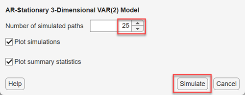
In the Simulations pane, a variable
SIM_VAR appears. This variable is a structure
array with the following fields:
Simulations— T-by-m-k array of simulated paths, with rows corresponding to in-sample times, columns corresponding to the variables in the model, and pages corresponding to the independently drawn pathsMean— T-by-m matrix of the pointwise average of the simulated paths for each variableUpperConfidenceBound— T-by-m matrix of upper confidence bounds of the pointwise 95% percentile-based confidence intervals for each pathLowerConfidenceBound— T-by-m matrix of lower confidence bounds of the pointwise 95% percentile-based confidence intervals for each path
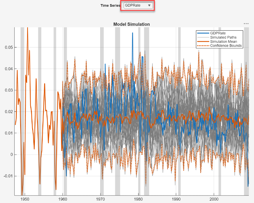
In the right pane, in the Sim(VAR) tab, is a
plot containing the following time series associated with the
GDPRate variable:
The time series data (thick blue line)
Each simulated path (thin gray lines)
The pointwise average of the simulated paths (thick orange line)
The pointwise 95% percentile-based confidence intervals (thick orange dashed line)
All simulated paths start at period two unless they require a longer presample to initialize the model, which is a common requirement for dynamic models. If a model requires a presample of more than 1 observation, all simulated paths begin at the time point after the end of the presample period. The length of the presample period depends on the dynamic model, see the associated reference page for details. A VAR(2) model requires two presample observations; therefore, all
simulated paths start at the third time period in the in-sample data. Because
M1SLRate observations begin at around 1960, the
simulated paths begin just after then.
Several GDP rates are more extreme than expected, and most rates before 1980 are above the mean, while most rates after 1990 are below the mean. These characteristics might suggest that the model does not capture the true data-generating process well enough.
Plot the TB3MS_Diff simulated paths and statistics.
In the right pane, in the Sim(VAR) window, click
Time Series >
TB3MS_Diff.
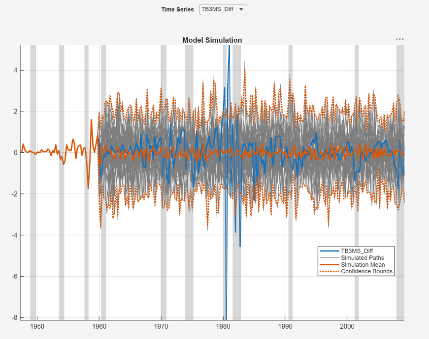
The change in the 3-month treasury bill shows unmodeled volatility in the early 1980s; the rest of the series is as expected give the model.