Create Model

Specify the AR(2) model

where the innovation process is Gaussian with variance 0.1.

Mdl = arima('Constant',0.5,'AR',{0.7 0.25},'Variance',.1);

Generate One Sample Path

Generate one sample path (with 50 observations) from the specified model, and plot.

rng(5)
Y = simulate(Mdl,50);

figure
plot(Y)
xlim([0,50])
title('Simulated AR(2) Process')

Because presample data was not specified, simulate sets the two required presample observations equal to the unconditional mean of the process

The unconditional variance of the process is

Compute the unconditional mean and variance of the process.

c = Mdl.Constant;
phi = Mdl.AR;
sigmaEps2 = Mdl.Variance;
mu = c/(1-phi{1}-phi{2})

mu = 
10.0000

sigma2 = (1-phi{2})/(1+phi{2})*sigmaEps2/((1-phi{2})^2 - phi{1}^2)

sigma2 = 
0.8276

Generate Many Sample Paths

Generate 1000 sample paths, each with 50 observations.

Y = simulate(Mdl,50,'NumPaths',1000);

figure
subplot(2,1,1)
plot(Y,'Color',[.85,.85,.85])
title('Simulated AR(2) Process')
hold on
h = plot(mean(Y,2),'k','LineWidth',2);
legend(h,'Simulation Mean','Location','NorthWest')
hold off
subplot(2,1,2)
plot(var(Y,0,2),'r','LineWidth',2)
title('Process Variance')
hold on
plot(1:50,sigma2*ones(50,1),'k--','LineWidth',1.5)
legend('Simulation','Theoretical',...
       'Location','SouthEast')
hold off

The simulation mean is constant over time. This is consistent with the definition of a stationary process. The process variance is not constant over time, however. There are transient effects at the beginning of the simulation due to the absence of presample data.

Around observation 50, the simulated variance approaches the theoretical variance.

Oversample to Reduce Transient Effects

To reduce transient effects, one option is to oversample the process. For example, to sample 50 observations, you can generate paths with more than 50 observations, and discard all but the last 50 observations as burn-in. Here, simulate paths of length 150, and discard the first 100 observations.

Y = simulate(Mdl,150,'NumPaths',1000);
Y = Y(101:end,:);

figure
subplot(2,1,1)
plot(Y,'Color',[.85,.85,.85])
title('Simulated AR(2) Process')
hold on
h = plot(mean(Y,2),'k','LineWidth',2);
legend(h,'Simulation Mean','Location','NorthWest')
hold off
subplot(2,1,2)
plot(var(Y,0,2),'r','LineWidth',2)
xlim([0,50])
title('Process Variance')
hold on
plot(1:50,sigma2*ones(50,1),'k--','LineWidth',1.5)
legend('Simulation','Theoretical',...
       'Location','SouthEast')
hold off

The realizations now look like draws from a stationary stochastic process. The simulation variance fluctuates (due to Monte Carlo error) around the theoretical variance.

Create Model

Specify the MA(12) model

where the innovation distribution is Gaussian with variance 0.2.

Mdl = arima('Constant',0.5,'MA',{0.8,0.2},...
    'MALags',[1,12],'Variance',0.2);

Generate Sample Paths

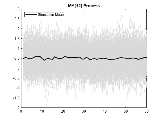
Generate 200 sample paths, each with 60 observations.

rng(5)
Y = simulate(Mdl,60,'NumPaths',200);

figure
plot(Y,'Color',[.85,.85,.85])
hold on
h = plot(mean(Y,2),'k','LineWidth',2);
legend(h,'Simulation Mean','Location','NorthWest')
title('MA(12) Process')
hold off

For an MA process, the constant term is the unconditional mean. The simulation mean is approximately $\mathit{c}$ = 0.5.

Plot Simulation Variance

The unconditional variance of the process is

Compute the unconditional variance.

theta = cell2mat(Mdl.MA);
sigmaEps2 = Mdl.Variance;
sigma2 = (1+sum(theta.^2))*sigmaEps2

sigma2 = 
0.3360

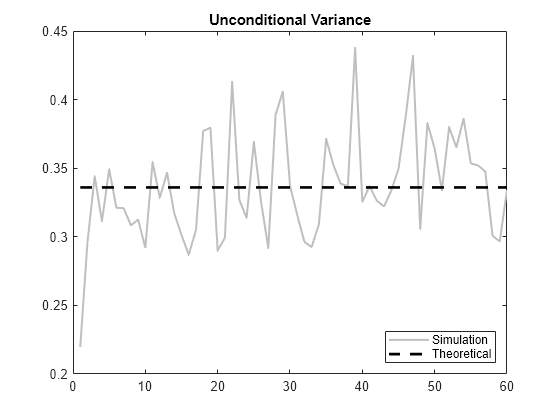
Because the model is stationary, the unconditional variance should be constant across all times. Plot the simulation variance, and compare it to the theoretical variance.

figure
plot(var(Y,0,2),'Color',[.75,.75,.75],'LineWidth',1.5)
xlim([0,60])
title('Unconditional Variance')
hold on
plot(1:60,sigma2*ones(60,1),'k--','LineWidth',2)
legend('Simulation','Theoretical',...
       'Location','SouthEast')
hold off

There appears to be a short burn-in period at the beginning of the simulation. During this time, the simulation variance is lower than expected. Afterwards, the simulation variance fluctuates around the theoretical variance.

Generate Many Sample Paths

Simulate 10,000 paths from the model, each with length 1000. Plot the simulation variance.

YM = simulate(Mdl,1000,'NumPaths',10000);
figure
plot(var(YM,0,2),'Color',[.75,.75,.75],'LineWidth',1.5)
ylim([0.3,0.36])
title('Unconditional Variance')
hold on
plot(1:1000,sigma2*ones(1000,1),'k--','LineWidth',2)
legend('Simulation','Theoretical',...
       'Location','SouthEast')
hold off

The Monte Carlo error is reduced when more realizations are generated. There is much less variability in the simulation variance, which tightly fluctuates around the theoretical variance.