Time Series Regression VII: Forecasting

Introduction

Many regression models in economics are built for explanatory purposes, to understand the interrelationships among relevant economic factors. The structure of these models is usually suggested by theory. Specification analysis compares various extensions and restrictions of the model to evaluate the contributions of individual predictors. Significance tests are especially important in these analyses. The modeling goal is to achieve a well-specified, accurately calibrated description of important dependencies. A reliable explanatory model might be used to inform planning and policy decisions by identifying factors to be considered in more qualitative analyses.

Regression models are also used for quantitative forecasting. These models are typically built from an initial set (perhaps empty, perhaps quite large) of potentially relevant predictors. Exploratory data analysis and predictor selection techniques are especially important in these analyses. The modeling goal, in this case, is to accurately predict the future. A reliable forecasting model might be used to identify risk factors involved in investment decisions and their relationship to critical outcomes like future default rates.

It is important, in practice, to distinguish the type of regression model under study. If a forecasting model is built through exploratory analysis, its overall predictive capability can be evaluated, but not the significance of individual predictors. In particular, it is misleading to use the same data to construct a model and then to draw inferences about its components.

This example focuses on forecasting methods for multiple linear regression (MLR) models. The methods are inherently multivariate, predicting the response in terms of past and present values of the predictor variables. As such, the methods are essentially different from the minimum mean squared error (MMSE) methods used in univariate modeling, where forecasts are based on the self-history of a single series.

We begin by loading relevant data from the previous example Time Series Regression VI: Residual Diagnostics:

load Data_TSReg6

Conditional Forecasting

Regression models describe the response produced by, or conditional on, associated values of the predictor variables. If a model has successfully captured the essential dynamics of a data-generating process (DGP), it can be used to explore contingency scenarios where predictor data is postulated rather than observed.

Models considered in this series of examples have been calibrated and tested using predictor data X0, measured at time t, and response data y0, measured at time t + 1. The time shift in the data means that these models provide one-step-ahead point forecasts of the response, conditional on the predictors.

To forecast further into the future, the only adjustment necessary is to estimate the model with larger shifts in the data. For example, to forecast two steps ahead, response data measured at time t + 2 (y0(2:end)) could be regressed on predictor data measured at time t (X0(1:end-1)). Of course, previous model analyses would have to be revisited to assure reliability.

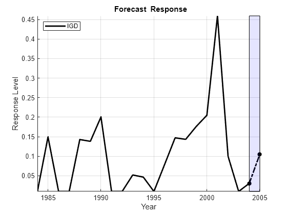
To illustrate, we use the M0 model to produce a conditional point forecast of the default rate in 2006, given new data on the predictors in 2005 provided in the variable X2005:

betaHat0 = M0.Coefficients.Estimate;
yHat0 = [1,X2005]*betaHat0;

D = dates(end);
Xm = min([X0(:);X2005']);
XM = max([X0(:);X2005']);

figure
hold on
plot(dates,X0,'LineWidth',2)
plot(D:D+1,[X0(end,:);X2005],'*-.','LineWidth',2)
fill([D D D+1 D+1],[Xm XM XM Xm],'b','FaceAlpha',0.1)
hold off
legend(predNames0,'Location','NW')
xlabel('Year') 
ylabel('Predictor Level') 
title('{\bf New Predictor Data}')
axis tight
grid on

Ym = min([y0;yHat0]);
YM = max([y0;yHat0]);

figure
hold on
plot(dates,y0,'k','LineWidth',2);
plot(D:D+1,[y0(end);yHat0],'*-.k','LineWidth',2)
fill([D D D+1 D+1],[Ym YM YM Ym],'b','FaceAlpha',0.1)
hold off
legend(respName0,'Location','NW')
xlabel('Year') 
ylabel('Response Level') 
title('{\bf Forecast Response}')
axis tight
grid on

We see that the SPR risk factor held approximately constant from 2004 to 2005, while modest decreases in the AGE and BBB risk factors were offset by a drop in CPF. CPF has a negative model coefficient, so the drop is associated with increased risk. The net result is a forecast jump in the default rate.

Unconditional Forecasting

In the absence of new predictor data (either measured or postulated), an unconditional forecast of the response may be desired.

One way to do this is to create a dynamic, univariate model of the response, such as an ARIMA model, independent of the predictors. ARIMA models depend on the existence of autocorrelations in the series from one time period to the next, which the model can exploit for forecasting purposes. ARIMA models are discussed elsewhere in the documentation.

Alternatively, a dynamic, multivariate model of the predictors can be built. This allows new values of the predictors to be forecast rather than observed. The regression model can then be used to forecast the response, conditional on the forecast of the predictors.

Robust multivariate forecasts are produced by vector autoregressive (VAR) models. A VAR model makes no structural assumptions about the form of the relationships among model variables. It posits only that every variable potentially influences every other. A system of dynamic regression equations is formed, with each variable appearing on the left-hand side of one equation, and the same lagged values of all of the variables, and possibly an intercept, appearing on the right-hand sides of all of the equations. The idea is to let the regression sort out which terms are actually significant.

For example, a VAR(3) model for the predictors in the default rate model would look like this:

The number of coefficients in the model is the number of variables times the number of autoregressive lags times the number of equations, plus the number of intercepts. Even with only a few variables, a model with a well-specified lag structure can grow quickly to a size that is untenable for estimation using small data samples.

Equation-by-equation OLS estimation performs well with VAR models, since each equation has the same regressors. This is true regardless of any cross-equation covariances that may be present in the innovations. Moreover, purely autoregressive estimation is numerically very stable.

The numerical stability of the estimates, however, relies on the stationarity of the variables being modeled. Differenced, stationary predictor variables lead to reliable forecasts of the differences. However, undifferenced predictor data may be required to forecast the response from the regression model. Integrating forecast differences has the potential to produce distorted forecast levels (see, for example, [2]). Nevertheless, the standard recommendation is to use stationary variables in the VAR, assuming that a short horizon will produce minimal reintegration errors.

VAR estimation and forecasting are carried out by the functions estimate and forecast. The following produces an unconditional point forecast of the default rate in 2005 from the M0 regression model:

% Estimate a VAR(1) model for the differenced predictors (with
% undifferenced |AGE|):

numLags = 1;
D1X0PreSample = D1X0(1:numLags,:);
D1X0Sample = D1X0(numLags+1:end,:);
numPreds0 = numParams0-1;
VARMdl = varm(numPreds0,numLags);
EstMdl = estimate(VARMdl,D1X0Sample,'Y0',D1X0PreSample);

% Forecast the predictors in D1X0:

horizon = 1;
ForecastD1X0 = forecast(EstMdl,horizon,D1X0);

% Integrate the differenced forecast to obtain the undifferenced forecast:

ForecastX0(1) = ForecastD1X0(1); % AGE
ForecastX0(2:4) = X0(end,2:4)+ForecastD1X0(2:4); % Other predictors

Xm = min([X0(:);ForecastX0(:)]);
XM = max([X0(:);ForecastX0(:)]);

figure
hold on
plot(dates,X0,'LineWidth',2)
plot(D:D+1,[X0(end,:);ForecastX0],'*-.','LineWidth',2)
fill([D D D+1 D+1],[Xm XM XM Xm],'b','FaceAlpha',0.1)
hold off
legend(predNames0,'Location','NW')
xlabel('Year') 
ylabel('Predictor Level')
title('{\bf Forecast Predictors}')
axis tight
grid on

% Forecast the response from the regression model:

ForecastY0 = [1,ForecastX0]*betaHat0;

Ym = min([y0;ForecastY0]);
YM = max([y0;ForecastY0]);

figure
hold on
plot(dates,y0,'k','LineWidth',2);
plot(D:D+1,[y0(end);ForecastY0],'*-.k','LineWidth',2)
fill([D D D+1 D+1],[Ym YM YM Ym],'b','FaceAlpha',0.1)
hold off
legend(respName0,'Location','NW')
xlabel('Year') 
ylabel('Response Level') 
title('{\bf Forecast Response}')
axis tight
grid on

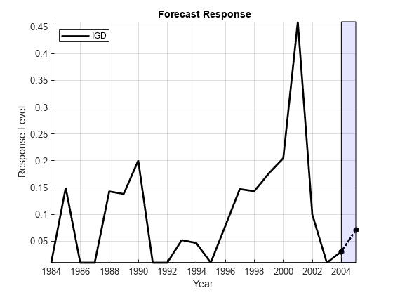
The result is an unconditional forecast that is similar to the conditional forecast made with actual 2005 data. The forecast depends on the number of lags used in the VAR model, numLags. The issue of choosing an appropriate lag length is addressed in the example Time Series Regression IX: Lag Order Selection.

The forecast generated by forecast is nonstochastic, in the sense that it uses zero-valued innovations outside of the sample. To generate a stochastic forecast, with specific structure in the innovations, use simulate or filter.

Forecast Error

Regardless of how new predictor data is acquired, forecasts from MLR models will contain errors. This is because MLR models, by their nature, forecast only expected values of the response. For example, the MLR model

forecasts $$y_{t+1}$$ using

Errors occur for two reasons:

$$•$$ The forecast does not incorporate the innovation $$e_{t+1}$$.

$$•$$ Sampling error produces a $$\underset{}{\overset{ˆ}{\beta }}$$ that is different from $$\beta$$.

As discussed in the example Time Series Regression II: Collinearity and Estimator Variance, the forecast error $${\underset{}{\overset{ˆ}{y}}}_{t+1}-y_{t+1}$$ is reduced if

$$•$$ The sample size is larger.

$$•$$ The variation of the predictors is larger.

$$•$$ $$X_{t+1}$$ is closer to its mean value.

The last item says that forecasts are improved when they are closer to the center of the distribution of sample values used to estimate the model. This leads to interval forecasts of nonconstant width.

Assuming normal, homoscedastic innovations, point forecasts can be converted to $N(y_{t+1}|X_t,{\sigma }^2)$ density and interval forecasts using standard formulas (see, for example, [1]). As discussed in the example Time Series Regression VI: Residual Diagnostics, however, standard formulas become biased and inefficient in the presence of autocorrelated or heteroscedastic innovations. In such situations, interval forecasts can be simulated using an appropriate series of innovations, but it is often recommended that a model be respecified to standardize the innovations as much as possible.

It is common to hold back a portion of the data for forecast evaluation, and estimate the model with an initial subsample. A basic performance test compares the root mean square error (RMSE) of out-of-subsample forecasts to the RMSE of a simple, baseline forecast that holds the last in-sample value of the response constant. If the model forecast does not significantly improve on the baseline forecast, then it is reasonable to suspect that the model has not abstracted the relevant economic forces in the DGP.

For example, the following tests the performance of the M0 model:

numTest = 3; % Number of observations held out for testing

% Training model:
X0Train = X0(1:end-numTest,:);
y0Train = y0(1:end-numTest);
M0Train = fitlm(X0Train,y0Train);

% Test set:
X0Test = X0(end-numTest+1:end,:);
y0Test = y0(end-numTest+1:end);

% Forecast errors:
y0Pred = predict(M0Train,X0Test);
DiffPred = y0Pred-y0Test;
DiffBase = y0Pred-y0(end-numTest);

% Forecast comparison:
RMSEPred = sqrt((DiffPred'*DiffPred)/numTest)

RMSEPred = 
0.1197

RMSEBase = sqrt((DiffBase'*DiffBase)/numTest)

RMSEBase = 
0.2945

The model forecast does show improvement relative to the baseline forecast. It is useful, however, to repeat the test with various values of numTest. This is complicated by the influential observation in 2001, three observations before the end of the data.

If a model passes the baseline test, it can be re-estimated with the full sample, as in M0. The test helps to distinguish the fit of a model from its ability to capture the dynamics of the DGP.

Summary

To generate new response values from a regression model, new values of the predictors are required. When new predictor values are postulated or observed, response data is extrapolated using the regression equation. For unconditional extrapolation, new predictor values must be forecast, as with a VAR model. The quality of predictions depends on both the in-sample fit of the model, and on the model's fidelity to the DGP.

The basic assumption of any forecasting model is that the economic data patterns described by the model will continue into the future. This is an assumption about the stability of the DGP. The social mechanisms driving economic processes, however, are never stable. The value of a forecasting model, especially one built by exploratory data analysis, can be short-lived. A basis in sound economic theory will improve the longevity of a model, but the volatile nature of the forecasting process must be acknowledged. This uncertainty is captured, to some degree, in models of the forecast error.

Econometric practice has shown that simple forecasting models often perform the best.

References

[1] Diebold, F. X. Elements of Forecasting. Mason, OH: Thomson Higher Education, 2007.
[2] Granger, C., and P. Newbold. "Forecasting Transformed Series." Journal of the Royal Statistical Society. Series B, Vol. 38, 1976, pp. 189–203.