irf

Generate vector error-correction (VEC) model impulse responses

Syntax

Response = irf(Mdl)

Response = irf(Mdl,Name,Value)

[Response,Lower,Upper] = irf(___)

Tbl = irf(___)

Description

The irf function returns the dynamic response, or the impulse response function (IRF), to a one-standard-deviation shock to each variable in a VEC(p – 1) model. A fully specified vecm model object characterizes the VEC model.

IRFs trace the effects of an innovation shock to one variable on the response of all variables in the system. In contrast, the forecast error variance decomposition (FEVD) provides information about the relative importance of each innovation in affecting all variables in the system. To estimate the FEVD of a VEC model characterized by a vecm model object, see fevd.

You can supply optional data, such as a presample, as a numeric array, table, or timetable. However, all specified input data must be the same data type. When the input model is estimated (returned by estimate), supply the same data type as the data used to estimate the model. The data type of the outputs matches the data type of the specified input data.

Response = irf(Mdl) returns a numeric array containing the orthogonalized IRF of the response variables that compose the VEC(p – 1) model Mdl characterized by a fully specified vecm model object. irf shocks variables at time 0, and returns the IRF for times 0 through 19.

If Mdl is an estimated model (returned by estimate) fit to a numeric matrix of input response data, this syntax applies.

example

Response = irf(Mdl,Name,Value) returns numeric arrays when all optional input data are numeric arrays. For example, irf(Mdl,NumObs=10,Method="generalized") specifies estimating a generalized IRF for 10 time points starting at time 0, during which irf applies the shock.

If Mdl is an estimated model (returned by estimate) fit to a numeric matrix of input response data, this syntax applies.

example

[Response,Lower,Upper] = irf(___) returns numeric arrays of lower Lower and upper Upper 95% confidence bounds for confidence intervals on the true IRF, for each period and variable in the IRF, using any input argument combination in the previous syntaxes. By default, irf estimates confidence bounds by conducting Monte Carlo simulation.

If Mdl is an estimated model fit to a numeric matrix of input response data, this syntax applies.

If Mdl is a custom vecm model object (an object not returned by estimate or modified after estimation), irf can require a sample size for the simulation SampleSize or presample responses Y0.

example

Tbl = irf(___) returns the table or timetable Tbl containing the IRFs and, optionally, corresponding 95% confidence bounds, of the response variables that compose the VEC(p – 1) model Mdl. The IRF of the corresponding response is a variable in Tbl containing a matrix with columns corresponding to the variables in the system shocked at time 0. (since R2022b)

If you set at least one name-value argument that controls the 95% confidence bounds on the IRF, Tbl also contains a variable for each of the lower and upper bounds. For example, Tbl contains confidence bounds when you set the NumPaths name-value argument.

If Mdl is an estimated model fit to a table or timetable of input response data, this syntax applies.

example

Examples

collapse all

Specify Data in Numeric Matrix When Plotting IRF

Open Live Script

Fit a 4-D VEC(2) model with two cointegrating relations to Danish money and income rate series data in a numeric matrix. Then, estimate the orthogonalized IRF from the estimated model.

Load the Danish money and income data set.

load Data_JDanish

The data set includes four time series in the table DataTable. For more details on the data set, enter Description at the command line.

Create a vecm model object that represents a 4-D VEC(2) model with two cointegrating relations. Specify the variable names.

Mdl = vecm(4,2,2);
Mdl.SeriesNames = DataTable.Properties.VariableNames;

Mdl is a vecm model object specifying the structure of a 4-D VEC(2) model; it is a template for estimation.

Fit the VEC(2) model to the numeric matrix of time series data Data.

EstMdl = estimate(Mdl,Data);

Mdl is a fully specified vecm model object representing an estimated 4-D VEC(2) model.

Estimate the orthogonalized IRF from the estimated VEC(2) model.

Response = irf(EstMdl);

Response is a 20-by-4-by-4 array representing the IRF of Mdl. Rows correspond to consecutive time points from time 0 to 19, columns correspond to variables receiving a one-standard-deviation innovation shock at time 0, and pages correspond to responses of variables to the variable being shocked. Mdl.SeriesNames specifies the variable order.

Display the IRF of the bond rate (variable 3, IB) when the log of real income (variable 2, Y) is shocked at time 0.

Response(:,2,3)

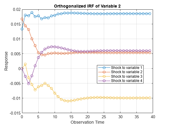
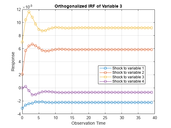
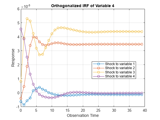
The armairf function plots the IRF of VAR models characterized by AR coefficient matrices. Plot the IRF of a VEC model by:

Expressing the VEC(2) model as a VAR(3) model by passing Mdl to varm
Passing the VAR model AR coefficients and innovations covariance matrix to armairf

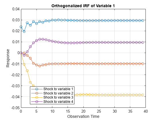
Plot the VEC(2) model IRF for 40 periods.

VARMdl = varm(EstMdl);
armairf(VARMdl.AR,[],InnovCov=VARMdl.Covariance, ...
    NumObs=40);

Figure contains an axes object. The axes object with title Orthogonalized IRF of Variable 1, xlabel Observation Time, ylabel Response contains 4 objects of type line. These objects represent Shock to variable 1, Shock to variable 2, Shock to variable 3, Shock to variable 4.

Figure contains an axes object. The axes object with title Orthogonalized IRF of Variable 2, xlabel Observation Time, ylabel Response contains 4 objects of type line. These objects represent Shock to variable 1, Shock to variable 2, Shock to variable 3, Shock to variable 4.

Figure contains an axes object. The axes object with title Orthogonalized IRF of Variable 3, xlabel Observation Time, ylabel Response contains 4 objects of type line. These objects represent Shock to variable 1, Shock to variable 2, Shock to variable 3, Shock to variable 4.

Figure contains an axes object. The axes object with title Orthogonalized IRF of Variable 4, xlabel Observation Time, ylabel Response contains 4 objects of type line. These objects represent Shock to variable 1, Shock to variable 2, Shock to variable 3, Shock to variable 4.

Each plot shows the four IRFs of a variable when all other variables are shocked at time 0. Mdl.SeriesNames specifies the variable order.

Estimate Generalized IRF of VEC Model

Open Live Script

Consider the 4-D VEC(2) model with two cointegrating relations in Specify Data in Numeric Matrix When Plotting IRF. Estimate the generalized IRF of the system for 50 periods.

Load the Danish money and income data set, then estimate the VEC(2) model.

load Data_JDanish

Mdl = vecm(4,2,2);
Mdl.SeriesNames = DataTable.Properties.VariableNames;
Mdl = estimate(Mdl,DataTable.Series);

Estimate the generalized IRF from the estimated VEC(2) model.

Response = irf(Mdl,Method="generalized",NumObs=50);

Response is a 50-by-4-by-4 array representing the generalized IRF of Mdl.

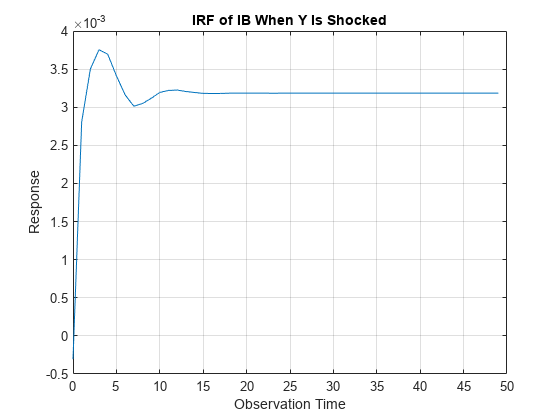
Plot the generalized IRF of the bond rate when real income is shocked at time 0.

figure;
plot(0:49,Response(:,2,3))
title("IRF of IB When Y Is Shocked")
xlabel("Observation Time")
ylabel("Response")
grid on

Figure contains an axes object. The axes object with title IRF of IB When Y Is Shocked, xlabel Observation Time, ylabel Response contains an object of type line.

When real income is shocked, the bond rate reacts and then settles at approximately 0.0032 after 15 periods.

Specify Data in Timetables When Computing IRF and Confidence Intervals

Since R2022b

Open Live Script

Fit a 4-D VEC(2) model with two cointegrating relations to Danish money and income rate series data in a numeric matrix. Then, estimate and plot the orthogonalized IRF and corresponding confidence intervals from the estimated model.

Load the Danish money and income data set.

load Data_JDanish

Create a vecm model object that represents a 4-D VEC(2) model with two cointegrating relations. Specify the variable names.

Mdl = vecm(4,2,2);
Mdl.SeriesNames = DataTable.Properties.VariableNames;

Mdl is a vecm model object specifying the structure of a 4-D VEC(2) model; it is a template for estimation.

Fit the VEC(2) model to the data set.

EstMdl = estimate(Mdl,DataTimeTable);

EstMdl is a fully specified vecm model object representing an estimated 4-D VEC(2) model.

Estimate the orthogonalized IRF and corresponding 95% confidence intervals from the estimated VEC(2) model. To return confidence intervals, you must set a name-value argument that controls confidence intervals, for example, Confidence. Set Confidence to 0.95.

rng(1); % For reproducibility
Tbl = irf(EstMdl,Confidence=0.95);
Tbl.Time(1)

ans = datetime
   01-Oct-1974

size(Tbl)

ans = 1×2

    20    12

Tbl is a timetable with 20 rows, representing the periods in the IRF, and 12 variables. Each variable is a 20-by-4 matrix of the IRF or confidence bound associated with a variable in the model EstMdl. For example, Tbl.M2_IRF(:,2) is the IRF of M2 resulting from a 1-standard-deviation shock on 01-Jul-1974 (period 0) to Mdl.SeriesNames(2), which is the variable Y. [Tbl.M2_IRF_LowerBound(:,2),Tbl.M2_IRF_UpperBound(:,2)] are the corresponding 95% confidence intervals. By default, irf uses the H1 Johansen form, which is the same default form that estimate uses.

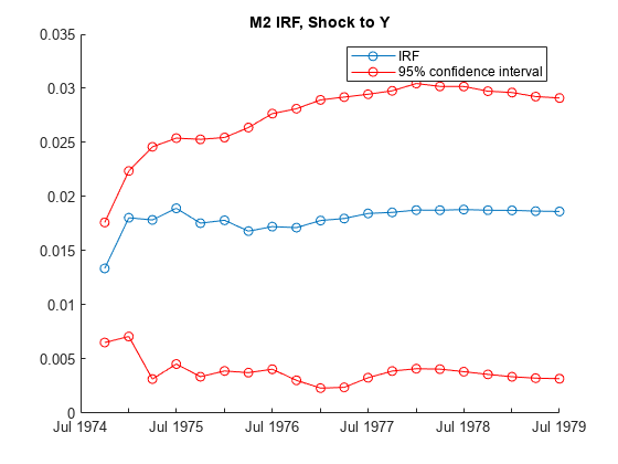
Plot the IRF of M2 and its 95% confidence interval resulting from a 1-standard-deviation shock on 01-Jul-1974 (period 0) to Mdl.SeriesNames(2), which is the variable Y.

idxM2 = startsWith(Tbl.Properties.VariableNames,"M2");
M2IRF = Tbl(:,idxM2);
shockIdx = 2;
figure
hold on
plot(M2IRF.Time,M2IRF.M2_IRF(:,shockIdx),"-o")
plot(M2IRF.Time,[M2IRF.M2_IRF_LowerBound(:,shockIdx) ...
    M2IRF.M2_IRF_UpperBound(:,shockIdx)],"-o",Color="r")
legend("IRF","95% confidence interval")
title('M2 IRF, Shock to Y')
hold off

Figure contains an axes object. The axes object with title M2 IRF, Shock to Y contains 3 objects of type line. These objects represent IRF, 95% confidence interval.

Monte Carlo Confidence Intervals on True IRF

Open Live Script

Consider the 4-D VEC(2) model with two cointegrating relations in Specify Data in Numeric Matrix When Plotting IRF. Estimate and plot its orthogonalized IRF and 95% Monte Carlo confidence intervals on the true IRF.

Load the Danish money and income data set, then estimate the VEC(2) model.

load Data_JDanish

Mdl = vecm(4,2,2);
Mdl.SeriesNames = DataTable.Properties.VariableNames;
Mdl = estimate(Mdl,DataTable.Series);

Estimate the IRF and corresponding 95% Monte Carlo confidence intervals from the estimated VEC(2) model.

rng(1); % For reproducibility
[Response,Lower,Upper] = irf(Mdl);

Response, Lower, and Upper are 20-by-4-by-4 arrays representing the orthogonalized IRF of Mdl and corresponding lower and upper bounds of the confidence intervals. For all arrays, rows correspond to consecutive time points from time 0 to 19, columns correspond to variables receiving a one-standard-deviation innovation shock at time 0, and pages correspond to responses of variables to the variable being shocked. Mdl.SeriesNames specifies the variable order.

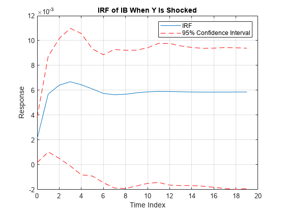
Plot the orthogonalized IRF with its confidence bounds of the bond rate when real income is shocked at time 0.

irfshock2resp3 = Response(:,2,3);
IRFCIShock2Resp3 = [Lower(:,2,3) Upper(:,2,3)];

figure;
h1 = plot(0:19,irfshock2resp3);
hold on
h2 = plot(0:19,IRFCIShock2Resp3,"r--");
legend([h1 h2(1)],["IRF" "95% Confidence Interval"])
xlabel("Time Index");
ylabel("Response");
title("IRF of IB When Y Is Shocked");
grid on
hold off

Figure contains an axes object. The axes object with title IRF of IB When Y Is Shocked, xlabel Time Index, ylabel Response contains 3 objects of type line. These objects represent IRF, 95% Confidence Interval.

When real income is shocked, the bond rate reacts and then settles between –0.002 and 0.0095 with 95% confidence.

Bootstrap Confidence Intervals on True IRF

Open Live Script

Consider the 4-D VEC(2) model with two cointegrating relations in Specify Data in Numeric Matrix When Plotting IRF. Estimate and plot its orthogonalized IRF and 90% bootstrap confidence intervals on the true IRF.

Load the Danish money and income data set, then estimate the VEC(2) model. Return the residuals from model estimation.

load Data_JDanish

Mdl = vecm(4,2,2);
Mdl.SeriesNames = DataTable.Properties.VariableNames;
[Mdl,~,~,Res] = estimate(Mdl,DataTable.Series);
T = size(DataTable,1) % Total sample size

T = 
55

n = size(Res,1)         % Effective sample size

n = 
52

Res is a 52-by-4 array of residuals. Columns correspond to the variables in Mdl.SeriesNames. The estimate function requires Mdl.P = 3 observations to initialize a VEC(2) model for estimation. Because presample data (Y0) is unspecified, estimate takes the first three observations in the specified response data to initialize the model. Therefore, the resulting effective sample size is T – Mdl.P = 52, and rows of Res correspond to the observation indices 4 through T.

Estimate the orthogonalized IRF and corresponding 90% bootstrap confidence intervals from the estimated VEC(2) model. Draw 500 paths of length n from the series of residuals.

rng(1) % For reproducibility
[Response,Lower,Upper] = irf(Mdl,E=Res,NumPaths=500, ...
    Confidence=0.9);

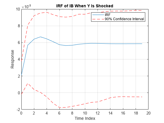
Plot the orthogonalized IRF with its confidence bounds of the bond rate when real income is shocked at time 0.

irfshock2resp3 = Response(:,2,3);
IRFCIShock2Resp3 = [Lower(:,2,3) Upper(:,2,3)];

figure;
h1 = plot(0:19,irfshock2resp3);
hold on
h2 = plot(0:19,IRFCIShock2Resp3,"r--");
legend([h1 h2(1)],["IRF" "90% Confidence Interval"])
xlabel("Time Index");
ylabel("Response");
title("IRF of IB When Y Is Shocked");
grid on
hold off

When real income is shocked, the bond rate reacts and then settles between approximately 0 and 0.010 with 90% confidence.

Input Arguments

collapse all

`Mdl` — VEC model
`vecm` model object

VEC model, specified as a vecm model object created by vecm or estimate. Mdl must be fully specified.

Name-Value Arguments

Specify optional pairs of arguments as Name1=Value1,...,NameN=ValueN, where Name is the argument name and Value is the corresponding value. Name-value arguments must appear after other arguments, but the order of the pairs does not matter.

Before R2021a, use commas to separate each name and value, and enclose Name in quotes.

Example: 'NumObs',10,'Method',"generalized" specifies estimating a generalized IRF for 10 time points starting at time 0, during which irf applies the shock, and ending at period 9.

Options for All IRFs

collapse all

`NumObs` — Number of periods
`20` (default) | positive integer

Number of periods for which irf computes the IRF, specified as a positive integer. NumObs specifies the number of observations to include in the IRF (the number of rows in Response or Tbl).

Example: NumObs=10 specifies the inclusion of 10 time points in the IRF starting at time 0, during which irf applies the shock, and ending at period 9.

Data Types: double

`Method` — IRF computation method
`"orthogonalized"` (default) | `"generalized"` | character vector

IRF computation method, specified as a value in this table.

Value	Description
`"orthogonalized"`	Compute impulse responses using orthogonalized, one-standard-deviation innovation shocks. `irf` uses the Cholesky factorization of `Mdl.Covariance` for orthogonalization.
`"generalized"`	Compute impulse responses using one-standard-deviation innovation shocks.

Example: Method="generalized"

Data Types: string | char

`Model` — Johansen form of VEC(p – 1) model deterministic terms
`"H1"` (default) | `"H2"` | `"H1"` | `"H"` | `"H"` | character vector

Johansen form of the VEC(p – 1) model deterministic terms [2], specified as a value in this table (for variable definitions, see Vector Error-Correction Model).

Value	Error-Correction Term	Description
`"H2"`	AB´y_{t − 1}	No intercepts or trends are present in the cointegrating relations, and no deterministic trends are present in the levels of the data. Specify this model only when all response series have a mean of zero.
`"H1*"`	A(B´y_t−1+c₀)	Intercepts are present in the cointegrating relations, and no deterministic trends are present in the levels of the data.
`"H1"`	A(B´y_t−1+c₀)+c₁	Intercepts are present in the cointegrating relations, and deterministic linear trends are present in the levels of the data.
`"H*"`	A(B´y_t−1+c₀+d₀t)+c₁	Intercepts and linear trends are present in the cointegrating relations, and deterministic linear trends are present in the levels of the data.
`"H"`	A(B´y_t−1+c₀+d₀t)+c₁+d₁t	Intercepts and linear trends are present in the cointegrating relations, and deterministic quadratic trends are present in the levels of the data. If quadratic trends are not present in the data, this model can produce good in-sample fits but poor out-of-sample forecasts.

For more details on the Johansen forms, see estimate.

If Mdl is an estimated vecm model object (an object returned by estimate and unmodified thereafter), the default is the Johansen form used for estimation (see 'Model').
Otherwise, the default is "H1".

Tip

A best practice is to maintain model consistency during the simulation that estimates confidence bounds. Therefore, if Mdl is an estimated vecm model object (an object returned by estimate and unmodified thereafter), incorporate any constraints imposed during estimation by deferring to the default value of Model.

Example: Model="H1*"

Data Types: string | char

Options for Confidence Bound Estimation

collapse all

`NumPaths` — Number of sample paths
`100` (default) | positive integer

Number of sample paths (trials) to generate, specified as a positive integer.

Example: NumPaths=1000 generates 1000 sample paths from which the software derives the confidence bounds.

Data Types: double

`SampleSize` — Number of observations for Monte Carlo simulation or bootstrap per sample path
positive integer

Number of observations for the Monte Carlo simulation or bootstrap per sample path, specified as a positive integer.

If Mdl is an estimated vecm model object (an object returned by estimate and unmodified thereafter), the default is the sample size of the data to which the model is fit (see summarize).
Otherwise:
- If irf estimates confidence bounds by conducting a Monte Carlo simulation, you must specify SampleSize.
- If irf estimates confidence bounds by bootstrapping residuals, the default is the length of the specified series of residuals (size(Res,1), where Res is the number of residuals in E or InSample).

Example: If you specify SampleSize=100 and do not specify the E name-value argument, the software estimates confidence bounds from NumPaths random paths of length 100 from Mdl.

Example: If you specify SampleSize=100,E=Res, the software resamples, with replacement, 100 observations (rows) from Res to form a sample path of innovations to filter through Mdl. The software forms NumPaths random sample paths from which it derives confidence bounds.

Data Types: double

`Y0` — Presample response data
numeric matrix

Presample response data that provides initial values for model estimation during the simulation, specified as a numpreobs-by-numseries numeric matrix. Use Y0 only in the following situations:

You supply other optional data inputs as numeric matrices.
Mdl is an estimated vecm model object (an object returned by estimate and unmodified thereafter) fit to a numeric matrix of response data.

numpreobs is the number of presample observations. numseries is Mdl.NumSeries, the dimensionality of the input model.

Each row is a presample observation, and measurements in each row occur simultaneously. The last row contains the latest presample observation. numpreobs is the number of specified presample responses and it must be at least Mdl.P. If you supply more rows than necessary, irf uses the latest Mdl.P observations only.

numseries is the dimensionality of the input VEC model Mdl.NumSeries. Columns must correspond to the response variables in Mdl.SeriesNames.

The following situations determine the default or whether presample response data is required.

If Mdl is an unmodified estimated model, irf sets Y0 to the presample response data used for estimation by default (see the Y0 name-value argument of estimate).
If Mdl is a custom model and you return confidence bounds Lower or Upper, you must specify Y0.

Data Types: double

`Presample` — Presample data
table | timetable

Since R2022b

Presample data that provide initial values for the model Mdl, specified as a table or timetable with numprevars variables and numpreobs rows. Use Presample only in the following situations:

You supply other optional data inputs as tables or timetables.
Mdl is an estimated vecm model object (an object returned by estimate and unmodified thereafter) fit to a numeric matrix of response data.

Each variable is a numpreobs numeric vector representing one path. To control presample variable selection, see the optional PresampleResponseVariables name-value argument.

If Presample is a timetable, all the following conditions must be true:

Presample must represent a sample with a regular datetime time step (see isregular).
The datetime vector of sample timestamps Presample.Time must be ascending or descending.

If Presample is a table, the last row contains the latest presample observation.

The following situations determine the default or whether presample response data is required.

If Mdl is an unmodified estimated model, irf sets Presample to the presample response data used for estimation by default (see the Presample name-value argument of estimate).
If Mdl is a custom model (for example, you modify a model after estimation by using dot notation) and you return confidence bounds in the table or timetable Tbl, you must specify Presample.

`PresampleResponseVariables` — Variables to select from `Presample` to use for presample response data
string vector | cell vector of character vectors | vector of integers | logical vector

Since R2022b

Variables to select from Presample to use for presample data, specified as one of the following data types:

String vector or cell vector of character vectors containing numseries variable names in Presample.Properties.VariableNames
A length numseries vector of unique indices (integers) of variables to select from Presample.Properties.VariableNames
A length numprevars logical vector, where PresampleResponseVariables(j) = true selects variable j from Presample.Properties.VariableNames, and sum(PresampleResponseVariables) is numseries

PresampleResponseVariables applies only when you specify Presample.

The selected variables must be numeric vectors and cannot contain missing values (NaN).

PresampleResponseNames does not need to contain the same names as in Mdl.SeriesNames; irf uses the data in selected variable PresampleResponseVariables(j) as a presample for Mdl.SeriesNames(j).

If the number of variables in Presample matches Mdl.NumSeries, the default specifies all variables in Presample. If the number of variables in Presample exceeds Mdl.NumSeries, the default matches variables in Presample to names in Mdl.SeriesNames.

Example: PresampleResponseVariables=["GDP" "CPI"]

Example: PresampleResponseVariables=[true false true false] or PresampleResponseVariable=[1 3] selects the first and third table variables for presample data.

Data Types: double | logical | char | cell | string

`X` — Predictor data
numeric matrix

Predictor data x_t for estimating the model regression component during the simulation, specified as a numeric matrix containing numpreds columns. Use X only in the following situations:

You supply other optional data inputs as tables or timetables.
Mdl is an estimated vecm model object (an object returned by estimate and unmodified thereafter) fit to a numeric matrix of response data.

numpreds is the number of predictor variables (size(Mdl.Beta,2)).

Each row corresponds to an observation, and measurements in each row occur simultaneously. The last row contains the latest observation. X must have at least SampleSize rows. If you supply more rows than necessary, irf uses only the latest observations. irf does not use the regression component in the presample period.

Columns correspond to individual predictor variables. All predictor variables are present in the regression component of each response equation.

To maintain model consistency when irf estimates the confidence bounds, a good practice is to specify predictor data when Mdl has a regression component. If Mdl is an estimated model, specify the predictor data used during model estimation (see the X name-value argument of estimate).

By default, irf excludes the regression component from confidence bound estimation, regardless of its presence in Mdl.

Data Types: double

`E` — Series of residuals from which to draw bootstrap samples
numeric matrix

Series of residuals from which to draw bootstrap samples, specified as a numperiods-by-numseries numeric matrix. irf assumes that E is free of serial correlation. Use E only in the following situations:

You supply other optional data inputs as numeric matrices.
Mdl is an estimated vecm model object (an object returned by estimate and unmodified thereafter) fit to a numeric matrix of response data.

Each column is the residual series corresponding to the response series names in Mdl.SeriesNames.

Each row corresponds to a period in the FEVD and the corresponding confidence bounds.

If Mdl is an estimated vecm model object (an object returned by estimate), you can specify E as the inferred residuals from estimation (see the E output argument of estimate or infer).

By default, irf derives confidence bounds by conducting a Monte Carlo simulation.

Data Types: double

`InSample` — Time series data
table | timetable

Since R2022b

Time series data containing numvars variables, including numseries variables of residuals e_t to bootstrap or numpreds predictor variables x_t for the model regression component, specified as a table or timetable. Use InSample only in the following situations:

You supply other optional data inputs as tables or timetables.
Mdl is an estimated vecm model object (an object returned by estimate and unmodified thereafter) fit to response data in a table or timetable.

Each variable is a single path of observations, which irfapplies to all NumPaths sample paths. If you specify Presample you must specify which variables are residuals and predictors, see the ResidualVariables and PredictorVariables name-value arguments.

Each row is an observation, and measurements in each row occur simultaneously. InSample must have at least SampleSize rows. If you supply more rows than necessary, irf uses only the latest observations.

If InSample is a timetable, the following conditions apply:

InSample must represent a sample with a regular datetime time step (see isregular).
The datetime vector InSample.Time must be strictly ascending or descending.
Presample must immediately precede InSample, with respect to the sampling frequency.

If InSample is a table, the last row contains the latest observation.

By default, irf derives confidence bounds by conducting a Monte Carlo simulation and does not use model the regression component, regardless of its presence in Mdl.

`ResidualVariables` — Variables to select from `InSample` to treat as residuals e_t for bootstrapping
string vector | cell vector of character vectors | vector of integers | logical vector

Since R2022b

Variables to select from InSample to treat as residuals for bootstrapping, specified as one of the following data types:

String vector or cell vector of character vectors containing numseries variable names in InSample.Properties.VariableNames
A length numseries vector of unique indices (integers) of variables to select from InSample.Properties.VariableNames
A length numvars logical vector, where ResidualVariables(j) = true selects variable j from InSample.Properties.VariableNames, and sum(ResidualVariables) is numseries

Regardless, selected residual variable j is the residual series for Mdl.SeriesNames(j).

The selected variables must be numeric vectors and cannot contain missing values (NaN).

By default, irf derives confidence bounds by conducting a Monte Carlo simulation.

Example: ResidualVariables=["GDP_Residuals" "CPI_Residuals"]

Example: ResidualVariables=[true false true false] or ResidualVariable=[1 3] selects the first and third table variables as the disturbance variables.

Data Types: double | logical | char | cell | string

`PredictorVariables` — Variables to select from `InSample` to treat as exogenous predictor variables x_t
string vector | cell vector of character vectors | vector of integers | logical vector

Since R2022b

Variables to select from InSample to treat as exogenous predictor variables x_t, specified as one of the following data types:

String vector or cell vector of character vectors containing numpreds variable names in InSample.Properties.VariableNames
A length numpreds vector of unique indices (integers) of variables to select from InSample.Properties.VariableNames
A length numvars logical vector, where PredictorVariables(j) = true selects variable j from InSample.Properties.VariableNames, and sum(PredictorVariables) is numpreds

Regardless, selected predictor variable j corresponds to the coefficients Mdl.Beta(:,j).

PredictorVariables applies only when you specify InSample.

The selected variables must be numeric vectors and cannot contain missing values (NaN).

By default, irf excludes the regression component, regardless of its presence in Mdl.

Example: PredictorVariables=["M1SL" "TB3MS" "UNRATE"]

Example: PredictorVariables=[true false true false] or PredictorVariable=[1 3] selects the first and third table variables as the response variables.

Data Types: double | logical | char | cell | string

`Confidence` — Confidence level
`0.95` (default) | numeric scalar in [0,1]

Confidence level for the confidence bounds, specified as a numeric scalar in the interval [0,1].

For each period, randomly drawn confidence intervals cover the true response 100*Confidence% of the time.

The default value is 0.95, which implies that the confidence bounds represent 95% confidence intervals.

Example: Confidence=0.9 specifies 90% confidence intervals.

Data Types: double

Note

NaN values in Y0, X, and E indicate missing data. irf removes missing data from these arguments by list-wise deletion. For each argument, if a row contains at least one NaN, irf removes the entire row.
List-wise deletion reduces the sample size, can create irregular time series, and can cause E and X to be unsynchronized.
irf issues an error when any table or timetable input contains missing values.

Output Arguments

collapse all

`Response` — IRF
numeric array

IRF of each variable, returned as a numobs-by-numseries-by-numseries numeric array. numobs is the value of NumObs. Columns and pages correspond to the response variables in Mdl.SeriesNames.

irf returns Response only in the following situations:

You supply optional data inputs as numeric matrices.
Mdl is an estimated model fit to a numeric matrix of response data.

Response(t + 1,j,k) is the impulse response of variable k at time t, attributable to a one-standard-deviation innovation shock applied at time 0 to variable j, for t = 0, 1, ..., numObs – 1, j = 1,2,...,numseries, and k = 1,2,...,numseries. For example, Response(1,2,3) is the impulse response of variable Mdl.SeriesName(3) at time t = 0, attributable to an innovation shock applied at time 0 to Mdl.SeriesName(2).

`Lower` — Lower confidence bounds
numeric array

Lower confidence bounds, returned as a numobs-by-numseries-by-numseries numeric array. Elements of Lower correspond to elements of Response.

irf returns Lower only in the following situations:

You supply optional data inputs as numeric matrices.
Mdl is an estimated model fit to a numeric matrix of response data.

Lower(t + 1,j,k) is the lower bound of the 100*Confidence-th percentile interval on the true impulse response of variable k at time t, attributable to a one-standard-deviation innovation shock applied at time 0 to variable j. For example, Lower(1,2,3) is the lower bound of the confidence interval on the true impulse response of variable Mdl.SeriesName(3) at time t = 0, attributable to an innovation shock applied at time 0 to Mdl.SeriesName(2).

`Upper` — Upper confidence bounds
numeric array

Upper confidence bounds, returned as a numobs-by-numseries-by-numseries numeric array. Elements of Upper correspond to elements of Response.

irf returns Upper only in the following situations:

You supply optional data inputs as numeric matrices.
Mdl is an estimated model fit to a numeric matrix of response data.

Upper(t + 1,j,k) is the upper bound of the 100*Confidence-th percentile interval on the true impulse response of variable k attime t, attributable to a one-standard-deviation innovation shock applied at time 0 to variable j. For example, Upper(1,2,3) is the upper bound of the confidence interval on the true impulse response of variable Mdl.SeriesName(3) at time t = 0, attributable to an innovation shock applied at time 0 to Mdl.SeriesName(2).

`Tbl` — IRF and confidence bounds
table | timetable

Since R2022b

IRF and confidence bounds, returned as a table or timetable with numobs rows. irf returns Tbl only in the following situations:

You supply optional data inputs as tables or timetables.
Mdl is an estimated model fit to response data in a table or timetable.

Regardless, the data type of Tbl is the same as the data type of specified data.

Tbl contains the following variables:

The IRF of each series in y_t. Each IRF variable in Tbl is a numobs-by-numseries numeric matrix, where numobs is the value of NumObs and numseries is the value of Mdl.NumSeries. irf names the IRF of response variable ResponseJ in Mdl.SeriesNames ResponseJ_IRF. For example, if Mdl.Series(j) is GDP, Tbl contains a variable for the corresponding IRF with the name GDP_IRF.
ResponseJ_IRF(t + 1,k) is the impulse response of variable ResponseJ at time t, attributable to a one-standard-deviation innovation shock applied at time 0 to variable k, for t = 0,1, ...,numObs – 1, J = 1,2,...,numseries, and k = 1,2,...,numseries.
The lower and upper confidence bounds on the true IRF of the response series, when you set at least one name-value argument that controls the confidence bounds. Each confidence bound variable in Tbl is a numobs-by-numseries numeric matrix. ResponseJ_IRF_LowerBound and ResponseJ_IRF_UpperBound are the names of the lower and upper bound variables, respectively, of the confidence interval on the IRF of response variable Mdl.SeriesNames(J) = ResponseJ. For example, if Mdl.SeriesNames(j) is GDP, Tbl contains variables for the corresponding lower and upper bounds of the confidence interval with the name GDP_IRF_LowerBound and GDP_IRF_UpperBound.
(ResponseJ_IRF_LowerBound(t,k), ResponseJ_IRF_UpperBound(t,k)) is the 100*Confidence-th percentile confidence interval on the IRF of response variable ResponseJ at time t, attributable to a one-standard-deviation innovation shock applied at time 0 to variable k, for t = 0,1,…,numobs – 1, J = 1,2,...,numseries, and k = 1,2,...,numseries.

If Tbl is a timetable, the row order of Tbl, either ascending or descending, matches the row order of InSample, when you specify it. If you do not specify InSample and you specify Presample, the row order of Tbl is the same as the row order of Presample.

More About

collapse all

Impulse Response Function

An impulse response function (IRF) of a time series model (or dynamic response of the system) measures the changes in the future responses of all variables in the system when a variable is shocked by an impulse. In other words, the IRF at time t is the derivative of the responses at time t with respect to an innovation at time t₀ (the time that innovation was shocked), t ≥ t₀.

Consider a numseries-D VEC(p – 1) model for the multivariate response variable y_t. In lag operator notation, the equivalent VAR(p) representation of a VEC(p – 1) model is:

$Γ (L) y_{t} = c + d t + β x_{t} + ε_{t},$

where $Γ (L) = I - Γ_{1} L - Γ_{2} L^{2} - ... - Γ_{p} L^{p}$ and I is the numseries-by-numseries identity matrix.

In lag operator notation, the infinite lag MA representation of y_t is:

$\begin{matrix} y_{t} = Γ^{- 1} (L) (c + β x_{t} + d t) + Γ^{- 1} (L) ε_{t} \\ = Ω (L) (c + β x_{t} + d t) + Ω (L) ε_{t} . \end{matrix}$

The general form of the IRF of y_t shocked by an impulse to variable j by one standard deviation of its innovation m periods into the future is:

$ψ_{j} (m) = C_{m} e_{j} .$

e_j is a selection vector of length numseries containing a 1 in element j and zeros elsewhere.
For the orthogonalized IRF, $C_{m} = Ω_{m} P,$ where P is the lower triangular factor in the Cholesky factorization of Σ, and Ω_m is the lag m coefficient of Ω(L).
For the generalized IRF, $C_{m} = σ_{j}^{- 1} Ω_{m} Σ,$ where σ_j is the standard deviation of innovation j.
The IRF is free of the model constant, regression component, and time trend.

Vector Error-Correction Model

A vector error-correction (VEC) model is a multivariate, stochastic time series model consisting of a system of m = numseries equations of m distinct, differenced response variables. Equations in the system can include an error-correction term, which is a linear function of the responses in levels used to stabilize the system. The cointegrating rank r is the number of cointegrating relations that exist in the system.

Each response equation can include an autoregressive polynomial composed of first differences of the response series (short-run polynomial of degree p – 1), a constant, a time trend, exogenous predictor variables, and a constant and time trend in the error-correction term.

A VEC(p – 1) model in difference-equation notation and in reduced form can be expressed in two ways:

This equation is the component form of a VEC model, where the cointegration adjustment speeds and cointegration matrix are explicit, whereas the impact matrix is implied.
$\begin{matrix} Δ y_{t} = A (B' y_{t - 1} + c_{0} + d_{0} t) + c_{1} + d_{1} t + Φ_{1} Δ y_{t - 1} + ... + Φ_{p - 1} Δ y_{t - (p - 1)} + β x_{t} + ε_{t} \\ = c + d t + A B' y_{t - 1} + Φ_{1} Δ y_{t - 1} + ... + Φ_{p - 1} Δ y_{t - (p - 1)} + β x_{t} + ε_{t} . \end{matrix}$
The cointegrating relations are B'y_{t
– 1} + c₀ + d₀t and the error-correction term is A(B'y_{t
– 1} + c₀ + d₀t).
This equation is the impact form of a VEC model, where the impact matrix is explicit, whereas the cointegration adjustment speeds and cointegration matrix are implied.
$\begin{matrix} Δ y_{t} = Π y_{t - 1} + A (c_{0} + d_{0} t) + c_{1} + d_{1} t + Φ_{1} Δ y_{t - 1} + ... + Φ_{p - 1} Δ y_{t - (p - 1)} + β x_{t} + ε_{t} \\ = c + d t + Π y_{t - 1} + Φ_{1} Δ y_{t - 1} + ... + Φ_{p - 1} Δ y_{t - (p - 1)} + β x_{t} + ε_{t} . \end{matrix}$

In the equations:

y_t is an m-by-1 vector of values corresponding to m response variables at time t, where t = 1,...,T.
Δy_t = y_t – y_{t – 1}. The structural coefficient is the identity matrix.
r is the number of cointegrating relations and, in general, 0 < r < m.
A is an m-by-r matrix of adjustment speeds.
B is an m-by-r cointegration matrix.
Π is an m-by-m impact matrix with a rank of r.
c₀ is an r-by-1 vector of constants (intercepts) in the cointegrating relations.
d₀ is an r-by-1 vector of linear time trends in the cointegrating relations.
c₁ is an m-by-1 vector of constants (deterministic linear trends in y_t).
d₁ is an m-by-1 vector of linear time-trend values (deterministic quadratic trends in y_t).
c = Ac₀ + c₁ and is the overall constant.
d = Ad₀ + d₁ and is the overall time-trend coefficient.
Φ_j is an m-by-m matrix of short-run coefficients, where j = 1,...,p – 1 and Φ_{p – 1} is not a matrix containing only zeros.
x_t is a k-by-1 vector of values corresponding to k exogenous predictor variables.
β is an m-by-k matrix of regression coefficients.
ε_t is an m-by-1 vector of random Gaussian innovations, each with a mean of 0 and collectively an m-by-m covariance matrix Σ. For t ≠ s, ε_t and ε_s are independent.

Condensed and in lag operator notation, the system is

$\begin{matrix} Φ (L) (1 - L) y_{t} = A (B' y_{t - 1} + c_{0} + d_{0} t) + c_{1} + d_{1} t + β x_{t} + ε_{t} \\ = c + d t + A B' y_{t - 1} + β x_{t} + ε_{t} \end{matrix}$

where $Φ (L) = I - Φ_{1} - Φ_{2} - ... - Φ_{p - 1}$ , I is the m-by-m identity matrix, and Ly_t = y_{t – 1}.

If m = r, then the VEC model is a stable VAR(p) model in the levels of the responses. If r = 0, then the error-correction term is a matrix of zeros, and the VEC(p – 1) model is a stable VAR(p – 1) model in the first differences of the responses.

Algorithms

If Method is "orthogonalized", then the resulting IRF depends on the order of the variables in the time series model. If Method is "generalized", then the resulting IRF is invariant to the order of the variables. Therefore, the two methods generally produce different results.
If Mdl.Covariance is a diagonal matrix, then the resulting generalized and orthogonalized IRFs are identical. Otherwise, the resulting generalized and orthogonalized IRFs are identical only when the first variable shocks all variables (for example, all else being the same, both methods yield the same value of Response(:,1,:)).
The predictor data in X or InSample represents a single path of exogenous multivariate time series. If you specify X or InSample and the model Mdl has a regression component (Mdl.Beta is not an empty array), irf applies the same exogenous data to all paths used for confidence interval estimation.
irf conducts a simulation to estimate the confidence bounds Lower and Upper or associated variables in Tbl.
- If you do not specify residuals by supplying E or using InSample, irf conducts a Monte Carlo simulation by following this procedure:
  1. Simulate NumPaths response paths of length SampleSize from Mdl.
  2. Fit NumPaths models that have the same structure as Mdl to the simulated response paths. If Mdl contains a regression component and you specify predictor data by supplying X or using InSample, then irf fits the NumPaths models to the simulated response paths and the same predictor data (the same predictor data applies to all paths).
  3. Estimate NumPaths IRFs from the NumPaths estimated models.
  4. For each time point t = 0,…,NumObs, estimate the confidence intervals by computing 1 – Confidence and Confidence quantiles (upper and lower bounds, respectively).
- Otherwise, irf conducts a nonparametric bootstrap by following this procedure:
  1. Resample, with replacement, SampleSize residuals from E or InSample. Perform this step NumPaths times to obtain NumPaths paths.
  2. Center each path of bootstrapped residuals.
  3. Filter each path of centered, bootstrapped residuals through Mdl to obtain NumPaths bootstrapped response paths of length SampleSize.
  4. Complete steps 2 through 4 of the Monte Carlo simulation, but replace the simulated response paths with the bootstrapped response paths.

References

[1] Hamilton, James D. Time Series Analysis. Princeton, NJ: Princeton University Press, 1994.

[2] Johansen, S. Likelihood-Based Inference in Cointegrated Vector Autoregressive Models. Oxford: Oxford University Press, 1995.

[3] Juselius, K. The Cointegrated VAR Model. Oxford: Oxford University Press, 2006.

[4] Pesaran, H. H., and Y. Shin. "Generalized Impulse Response Analysis in Linear Multivariate Models." Economic Letters. Vol. 58, 1998, pp. 17–29.

Version History

Introduced in R2019a

expand all

R2022b: `irf` accepts input data in tables and timetables, and return results in tables and timetables

In addition to accepting input data in numeric arrays, irf accepts input data in tables and timetables. irf chooses default series on which to operate, but you can use the following name-value arguments to select variables.

Presample specifies the input table or regular timetable of presample response data.
PresampleResponseVariables specifies the response series names from Presample.
Insample specifies the table or regular timetable of residual and predictor data to compute bootstrap estimates.
ResidualVariables specifies the residual series names in InSample.
PredictorVariables specifies the predictor series in InSample for a model regression component.

irf

Syntax

Description

Examples

Specify Data in Numeric Matrix When Plotting IRF

Estimate Generalized IRF of VEC Model

Specify Data in Timetables When Computing IRF and Confidence Intervals

Monte Carlo Confidence Intervals on True IRF

Bootstrap Confidence Intervals on True IRF

Input Arguments

Mdl — VEC model vecm model object

Name-Value Arguments

NumObs — Number of periods 20 (default) | positive integer

Method — IRF computation method "orthogonalized" (default) | "generalized" | character vector

Model — Johansen form of VEC(p – 1) model deterministic terms "H1" (default) | "H2" | "H1*" | "H*" | "H" | character vector

NumPaths — Number of sample paths 100 (default) | positive integer

SampleSize — Number of observations for Monte Carlo simulation or bootstrap per sample path positive integer

Y0 — Presample response data numeric matrix

Presample — Presample data table | timetable

PresampleResponseVariables — Variables to select from Presample to use for presample response data string vector | cell vector of character vectors | vector of integers | logical vector

X — Predictor data numeric matrix

E — Series of residuals from which to draw bootstrap samples numeric matrix

InSample — Time series data table | timetable

ResidualVariables — Variables to select from InSample to treat as residuals et for bootstrapping string vector | cell vector of character vectors | vector of integers | logical vector

PredictorVariables — Variables to select from InSample to treat as exogenous predictor variables xt string vector | cell vector of character vectors | vector of integers | logical vector

Confidence — Confidence level 0.95 (default) | numeric scalar in [0,1]

Output Arguments

Response — IRF numeric array

Lower — Lower confidence bounds numeric array

Upper — Upper confidence bounds numeric array

Tbl — IRF and confidence bounds table | timetable

More About

Impulse Response Function

Vector Error-Correction Model

Algorithms

References

Version History

R2022b: irf accepts input data in tables and timetables, and return results in tables and timetables

See Also

Objects

Functions

`Mdl` — VEC model
`vecm` model object

`NumObs` — Number of periods
`20` (default) | positive integer

`Method` — IRF computation method
`"orthogonalized"` (default) | `"generalized"` | character vector

`Model` — Johansen form of VEC(p – 1) model deterministic terms
`"H1"` (default) | `"H2"` | `"H1"` | `"H"` | `"H"` | character vector

`NumPaths` — Number of sample paths
`100` (default) | positive integer

`SampleSize` — Number of observations for Monte Carlo simulation or bootstrap per sample path
positive integer

`Y0` — Presample response data
numeric matrix

`Presample` — Presample data
table | timetable

`PresampleResponseVariables` — Variables to select from `Presample` to use for presample response data
string vector | cell vector of character vectors | vector of integers | logical vector

`X` — Predictor data
numeric matrix

`E` — Series of residuals from which to draw bootstrap samples
numeric matrix

`InSample` — Time series data
table | timetable

`ResidualVariables` — Variables to select from `InSample` to treat as residuals e_t for bootstrapping
string vector | cell vector of character vectors | vector of integers | logical vector

`PredictorVariables` — Variables to select from `InSample` to treat as exogenous predictor variables x_t
string vector | cell vector of character vectors | vector of integers | logical vector

`Confidence` — Confidence level
`0.95` (default) | numeric scalar in [0,1]

`Response` — IRF
numeric array

`Lower` — Lower confidence bounds
numeric array

`Upper` — Upper confidence bounds
numeric array

`Tbl` — IRF and confidence bounds
table | timetable

R2022b: `irf` accepts input data in tables and timetables, and return results in tables and timetables