Main Content

fitSmoothingSpline

Fit smoothing spline to bond market data

Description

CurveObj = IRFunctionCurve.fitSmoothingSpline(Type,Settle,Instruments,Lambdafun) fits a smoothing spline to market data for a bond.

Note

You must have a license for Curve Fitting Toolbox™ software to use the fitSmoothingSpline method.

example

CurveObj = IRFunctionCurve.fitSmoothingSpline(___,Name,Value) adds optional name-value pair arguments.

example

Examples

collapse all

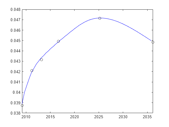
This example shows how to use a fitSmoothingSpline function to fit market data for a bond.

Settle = repmat(datenum('30-Apr-2008'),[6 1]);
Maturity = [datenum('07-Mar-2009');datenum('07-Mar-2011');...
datenum('07-Mar-2013');datenum('07-Sep-2016');...
datenum('07-Mar-2025');datenum('07-Mar-2036')];

CleanPrice = [100.1;100.1;100.8;96.6;103.3;96.3];
CouponRate = [0.0400;0.0425;0.0450;0.0400;0.0500;0.0425];
Instruments = [Settle Maturity CleanPrice CouponRate];
PlottingPoints = datenum('07-Mar-2009'):180:datenum('07-Mar-2036');
Yield = bndyield(CleanPrice,CouponRate,Settle,Maturity);

% Use the AUGKNT function to construct the knots for a cubic spline at
% every 5 years.
CustomKnots = augknt(0:5:30,4);
SmoothingModel = IRFunctionCurve.fitSmoothingSpline('Zero',datenum('30-Apr-2008'),...
Instruments,@(t) 1000,'knots', CustomKnots);

% Create the plot.
plot(datetime(PlottingPoints,"ConvertFrom","datenum"), getParYields(SmoothingModel, PlottingPoints),'b')
hold on
scatter(datetime(Maturity,"ConvertFrom","datenum"),Yield,'black')

Figure contains an axes object. The axes object contains 2 objects of type line, scatter.

This example shows for to use fitSmoothinSpline function to fit the interest-rate curve and model the Lambdafun penalty function.

First, load the data.

load ukdata20080430

Convert the repo rates to be equivalent zero coupon bonds.

RepoCouponRate = repmat(0,size(RepoRates));
RepoPrice = bndprice(RepoRates, RepoCouponRate, RepoSettle, RepoMaturity);

Aggregate the data.

Settle = [RepoSettle;BondSettle];
Maturity = [RepoMaturity;BondMaturity];
CleanPrice = [RepoPrice;BondCleanPrice];
CouponRate = [RepoCouponRate;BondCouponRate];
Instruments = [Settle Maturity CleanPrice CouponRate];
InstrumentPeriod = [repmat(0,6,1);repmat(2,31,1)];
CurveSettle = datenum('30-Apr-2008');

Choose the parameters for the Lambdafun input argument.

L = 9.2;
S = -1;
mu = 1;

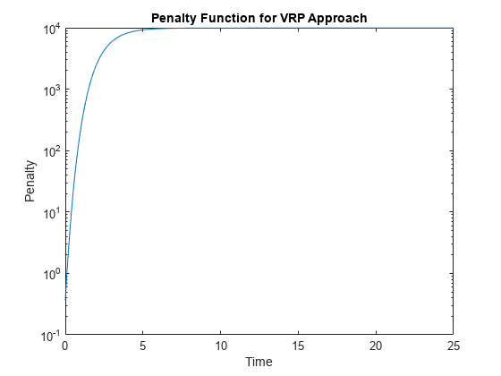
Define the Lambdafun penalty function.

lambdafun = @(t) exp(L - (L-S)*exp(-t/mu));
t = 0:.1:25;
y = lambdafun(t);
figure
semilogy(t,y);
title('Penalty Function for VRP Approach')
ylabel('Penalty')
xlabel('Time')

Figure contains an axes object. The axes object with title Penalty Function for VRP Approach, xlabel Time, ylabel Penalty contains an object of type line.

Use the fitSmoothinSpline function to fit the interest-rate curve and model the Lambdafun penalty function.

VRPModel = IRFunctionCurve.fitSmoothingSpline('Forward',CurveSettle,...
Instruments,lambdafun,'Compounding',-1, 'InstrumentPeriod',InstrumentPeriod)
VRPModel = 
			 Type: Forward
		   Settle: 733528 (30-Apr-2008)
	  Compounding: -1
			Basis: 0 (actual/actual)

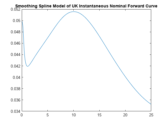
Plot the smoothing spline interest-rate curve for the forward rates.

PlottingDates = CurveSettle+20:30:CurveSettle+365*25;
TimeToMaturity = yearfrac(CurveSettle,PlottingDates);
VRPForwardRates = getForwardRates(VRPModel, PlottingDates);
figure;plot(TimeToMaturity,VRPForwardRates)
title('Smoothing Spline Model of UK Instantaneous Nominal Forward Curve')

Figure contains an axes object. The axes object with title Smoothing Spline Model of UK Instantaneous Nominal Forward Curve contains an object of type line.

Input Arguments

collapse all

Type of interest-rate curve for a bond, specified by using a scalar character vector.

Data Types: char

Settle date of interest-rate curve, specified serial date number or date character vector.

Data Types: double | char

Instruments, specified using an N-by-4 data matrix where the first column is Settle date using a serial date number, the second column is Maturity using a serial date number, the third column is the clean price, and the fourth column is a CouponRate for the bond.

Data Types: double

Penalty function, specified using a function handle. The penalty function that takes as its input time and returns a penalty value. The function handle for the penalty function takes one numeric input (time-to-maturity) and returns one numeric output (penalty to be applied to the curvature of the spline). For more information on defining a function handle, see the MATLAB® Programming Fundamentals documentation.

Note

The smoothing spline represents the forward curve. The spline is penalized for curvature by specifying a penalty function. This fit can only be done with a FitType of DurationWeightedPrice.

Data Types: function_handle

Name-Value Arguments

Specify optional pairs of arguments as Name1=Value1,...,NameN=ValueN, where Name is the argument name and Value is the corresponding value. Name-value arguments must appear after other arguments, but the order of the pairs does not matter.

Before R2021a, use commas to separate each name and value, and enclose Name in quotes.

Example: CurveObj = IRFunctionCurve.fitSmoothingSpline('Zero',datenum('30-Apr-2008'),Instruments,@(t) 1000,'Knots',CustomKnots)

Name-Value Pair Arguments for All Bond Instruments

collapse all

Compounding frequency per-year for the IRFunctionCurve object, specified as the comma-separated pair consisting of 'Compounding' and a scalar numeric using one of the supported values:

  • −1 = Continuous compounding

  • 0 = Simple interest (no compounding)

  • 1 = Annual compounding

  • 2 = Semiannual compounding

  • 3 = Compounding three times per year

  • 4 = Quarterly compounding

  • 6 = Bimonthly compounding

  • 12 = Monthly compounding

Data Types: double

Day count basis of the interest-rate curve, specified as the comma-separated pair consisting of 'Basis' and a scalar integer.

  • 0 — actual/actual

  • 1 — 30/360 (SIA)

  • 2 — actual/360

  • 3 — actual/365

  • 4 — 30/360 (PSA)

  • 5 — 30/360 (ISDA)

  • 6 — 30/360 (European)

  • 7 — actual/365 (Japanese)

  • 8 — actual/actual (ICMA)

  • 9 — actual/360 (ICMA)

  • 10 — actual/365 (ICMA)

  • 11 — 30/360E (ICMA)

  • 12 — actual/365 (ISDA)

  • 13 — BUS/252

For more information, see Basis.

Data Types: double

Knot locations (times-to-maturity), specified as the comma-separated pair consisting of 'Knots' and a vector. The default is for the spline type to be cubic but you can specify any spline type by explicitly specifying the knots. User-defined knots can be specified using the following Curve Fitting Toolbox command, where k is the order: augknt(knots,k).

Data Types: double

Name-Value Pair Arguments for Each Bond Instrument

collapse all

Coupons per year for the bond, specified as the comma-separated pair consisting of 'InstrumentPeriod' and a scalar numeric value.

Data Types: double

Day count basis of the bond, specified as the comma-separated pair consisting of 'InstrumentBasis' and a scalar integer.

  • 0 — actual/actual

  • 1 — 30/360 (SIA)

  • 2 — actual/360

  • 3 — actual/365

  • 4 — 30/360 (PSA)

  • 5 — 30/360 (ISDA)

  • 6 — 30/360 (European)

  • 7 — actual/365 (Japanese)

  • 8 — actual/actual (ICMA)

  • 9 — actual/360 (ICMA)

  • 10 — actual/365 (ICMA)

  • 11 — 30/360E (ICMA)

  • 12 — actual/365 (ISDA)

  • 13 — BUS/252

Note

InstrumentBasis distinguishes a bond instrument's Basis value from the interest-rate curve's Basis value.

For more information, see Basis.

Data Types: double

End-of-month rule, specified as the comma-separated pair consisting of 'InstrumentEndMonthRule' and a logical value. This rule applies only when Maturity is an end-of-month date for a month having 30 or fewer days.

  • 0 = ignore rule, meaning that a bond's coupon payment date is always the same numerical day of the month.

  • 1 = set rule on (default), meaning that a bond's coupon payment date is always the last actual day of the month.

Data Types: logical

Instrument issue date, specified as the comma-separated pair consisting of 'InstrumentIssueDate' and a scalar serial date number or date character vector.

Data Types: double | char

Date when a bond makes its first coupon payment (used when bond has an irregular first coupon period), specified as the comma-separated pair consisting of 'InstrumentFirstCouponDate' and a scalar serial date number or date character vector. When InstrumentFirstCouponDate and InstrumentLastCouponDate are both specified, InstrumentFirstCouponDate takes precedence in determining the coupon payment structure. If you do not specify a InstrumentFirstCouponDate, the cash flow payment dates are determined from other inputs.

Data Types: double | char

Last coupon date of a bond before the maturity date (used when bond has an irregular last coupon period), specified as the comma-separated pair consisting of 'InstrumentLastCouponDate' and a scalar serial date number or date character vector. In the absence of a specified InstrumentFirstCouponDate, a specified InstrumentLastCouponDate determines the coupon structure of the bond. The coupon structure of a bond is truncated at the InstrumentLastCouponDate, regardless of where it falls, and is followed only by the bond's maturity cash flow date. If you do not specify a InstrumentLastCouponDate, the cash flow payment dates are determined from other inputs.

Data Types: double | char

Face or par value, specified as the comma-separated pair consisting of 'InstrumentFace' and a scalar numeric.

Data Types: double

Note

When using Instrument name-value pairs, you can specify simple interest for a bond by specifying the InstrumentPeriod value as 0. If InstrumentBasis and InstrumentPeriod are not specified for a bond, the following default values are used: InstrumentBasis is 0 (act/act) and InstrumentPeriod is 2.

Output Arguments

collapse all

Smoothing spline curve model, returned as a structure.

Algorithms

The term structure can be modeled with a spline — specifically, one way to model the term structure is by representing the forward curve with a cubic spline. To ensure that the spline is sufficiently smooth, a penalty is imposed relating to the curvature (second derivative) of the spline:

where the first term is the difference between the observed price P and the predicted price, P^, (weighted by the bond's duration, D) summed over all bonds in our data set and the second term is the penalty term (where λ is a penalty function and f is the spline).

See [3], [4], [5] below.

There have been different proposals for the specification of the penalty function λ. One approach, advocated by [4], and currently used by the UK Debt Management Office, is a penalty function of the following form:

References

[1] Nelson, C.R., Siegel, A.F. “Parsimonious modelling of yield curves.” Journal of Business. Vol. 60, 1987, pp 473–89.

[2] Svensson, L.E.O. “Estimating and interpreting forward interest rates: Sweden 1992-4.” International Monetary Fund, IMF Working Paper, 1994/114.

[3] Fisher, M., Nychka, D., Zervos, D. “Fitting the term structure of interest rates with smoothing splines.” Board of Governors of the Federal Reserve System, Federal Reserve Board Working Paper 1995-1.

[4] Anderson, N., Sleath, J. “New estimates of the UK real and nominal yield curves.” Bank of England Quarterly Bulletin, November, 1999, pp 384–92.

[5] Waggoner, D. “Spline Methods for Extracting Interest Rate Curves from Coupon Bond Prices.” Federal Reserve Board Working Paper 1997–10.

[6] “Zero-coupon yield curves: technical documentation.” BIS Papers No. 25, October 2005.

[7] Bolder, D.J., Gusba, S. “Exponentials, Polynomials, and Fourier Series: More Yield Curve Modelling at the Bank of Canada.” Working Papers 2002–29, Bank of Canada.

[8] Bolder, D.J., Streliski, D. “Yield Curve Modelling at the Bank of Canada.” Technical Reports 84, 1999, Bank of Canada.

Version History

Introduced in R2008b