Pricing European and American Spread Options

Open Live Script

This example shows how to price and calculate sensitivities for European and American spread options using various techniques. First, the price and sensitivities for a European spread option is calculated using closed form solutions. Then, price and sensitivities for an American spread option is calculated using finite difference and Monte Carlo simulations. Finally, further analysis is conducted on spread options with a different range of inputs.

Spread options are options on the difference of two underlying asset prices. For example, a call option on the spread between two assets has the following payoff at maturity:

$m a x (X_{1} - X_{2} - K, 0)$

where $X_{1}$ is the price of the first underlying asset, $X_{2}$ is the price of the second underlying asset, and $K$ is the strike price. At maturity, if the spread $X_{1} - X_{2}$ is greater than the strike price $K$ , the option holder exercises the option and gains the difference between the spread and the strike price. If the spread is less than 0, the option holder does not exercise the option, and the payoff is 0. Spread options are frequently traded in the energy market. Two examples are:

Crack spreads: Options on the spread between refined petroleum products and crude oil. The spread represents the refinement margin made by the oil refinery by "cracking" the crude oil into a refined petroleum product.
Spark spreads: Options on the spread between electricity and some type of fuel. The spread represents the margin of the power plant, which takes fuel to run its generator to produce electricity.

Overview of the Pricing Methods

There are several methods to price spread options, as discussed in [1]. This example uses the closed form, finite difference, and Monte Carlo simulations to price spread options. The advantages and disadvantages of each method are discussed below:

Closed form solutions and approximations of partial differential equations (PDE) are advantageous because they are very fast, and extend well to computing sensitivities (Greeks). However, closed form solutions are not always available, for example for American spread options.
The finite difference method is a numerical procedure to solve PDEs by discretizing the price and time variables into a grid. A detailed analysis of this method can be found in [2]. It can handle cases where closed form solutions are not available. Also, finite difference extends well to calculating sensitivities because it outputs a grid of option prices for a range of underlying prices and times. However, it is slower than the closed form solutions.
Monte Carlo simulation uses random sampling to simulate movements of the underlying asset prices. It handles cases where closed solutions do not exist. However, it usually takes a long time to run, especially if sensitivities are calculated.

Pricing a European Spread Option

The following example demonstrates the pricing of a crack spread option.

A refiner is concerned about its upcoming maintenance schedule and needs to protect against decreasing crude oil prices and increasing heating oil prices. During the maintenance the refiner needs to continue providing customers with heating oil to meet their demands. The refiner's strategy is to use spread options to manage its hedge.

On January 2013, the refiner buys a 1:1 crack spread option by purchasing heating oil futures and selling crude oil futures. CLF14 WTI crude oil futures is at $100 per barrel and HOF14 heating oil futures contract is at $2.6190 per gallon.

clear;

% Price, volatility, and dividend of heating oil
Price1gallon = 2.6190;       % $/gallon 
Price1 = Price1gallon*42;    % $/barrel
Vol1 = 0.10;
Div1 = 0.03;

% Price, volatility, and dividend of WTI crude oil
Price2 = 100;     % $/barrel
Vol2 = 0.15;
Div2 = 0.02;

% Correlation of underlying prices
Corr = 0.3;

% Option type
OptSpec = 'call';

% Strike
Strike = 5;

% Settlement date
Settle = '01-Jan-2013';

% Maturity
Maturity = '01-Jan-2014'; 

% Risk free rate
RiskFreeRate = 0.05;

The pricing functions take an interest-rate term structure and stock structure as inputs. Also, you need to specify which outputs are of interest.

% Define RateSpec
Compounding = -1;
Basis = 1;
RateSpec = intenvset('ValuationDate', Settle, 'StartDates', Settle, ...
    'EndDates', Maturity, 'Rates', RiskFreeRate, 'Compounding', ...
    Compounding, 'Basis', Basis);

% Define StockSpec for the two assets
StockSpec1 = stockspec(Vol1, Price1, 'Continuous', Div1);
StockSpec2 = stockspec(Vol2, Price2, 'Continuous', Div2);

% Specify price and sensitivity outputs
OutSpec = {'Price', 'Delta', 'Gamma'};

The Financial Instruments Toolbox™ contains two types of closed form approximations for calculating price and sensitivities of European spread options: the Kirk's approximation (spreadbykirk, spreadsensbykirk) and the Bjerksund and Stensland model (spreadbybjs, spreadsensbybjs) [3].

The function spreadsensbykirk calculates prices and sensitivities for a European spread option using the Kirk's approximation.

% Kirk's approximation
[PriceKirk, DeltaKirk, GammaKirk] = ...
    spreadsensbykirk(RateSpec, StockSpec1, StockSpec2, Settle, ...
    Maturity, OptSpec, Strike, Corr, 'OutSpec', OutSpec)

PriceKirk = 
8.3636

DeltaKirk = 1×2

    0.6108   -0.5590

GammaKirk = 1×2

    0.0225    0.0249

The function spreadsensbybjs calculates the prices and sensitivities for a European spread option using the Bjerksund and Stensland model. In [3], Bjerksund and Stensland explains that the Kirk's approximation tends to underprice the spread option when the strike is close to zero, and overprice when the strike is further away from zero. In comparison, the model by Bjerksund and Stensland has higher precision.

% Bjerksund and Stensland model
[PriceBJS, DeltaBJS, GammaBJS] = ...
    spreadsensbybjs(RateSpec, StockSpec1, StockSpec2, Settle, ...
    Maturity, OptSpec, Strike, Corr, 'OutSpec', OutSpec)

PriceBJS = 
8.3662

DeltaBJS = 1×2

    0.6115   -0.5597

GammaBJS = 1×2

    0.0225    0.0248

A comparison of the calculated prices show that the two closed form models produce similar results for price and sensitivities. In addition to delta and gamma, the functions can also calculate theta, vega, lambda, and rho.

displayComparison('Kirk', 'BJS', PriceKirk, PriceBJS, DeltaKirk, DeltaBJS, GammaKirk, GammaBJS)

Comparison of prices:

Kirk:    8.363641
BJS :    8.366158

Comparison of delta:

Kirk:    0.610790     -0.558959
BJS :    0.611469     -0.559670

Comparison of gamma:

Kirk:    0.022533      0.024850
BJS :    0.022495      0.024819

Pricing an American Spread Option

Although the closed form approximations are fast and well suited for pricing European spread options, they cannot price American spread options. Using the finite difference method and the Monte Carlo method, an American spread option can be priced. In this example, an American spread option is priced with the same attributes as the above crack spread option.

The finite difference method numerically solves a PDE by discretizing the underlying price and time variables into a grid. The Financial Instrument Toolbox™ contains the functions spreadbyfd and spreadsensbyfd, which calculate prices and sensitivities for European and American spread options using the finite difference method. For the finite difference method, the composition of the grid has a large impact on the quality of the output and the execution time. Generally, a finely discretized grid will result in outputs that are closer to the theoretical value, but it comes at the cost of longer execution times. The composition of the grid is controlled using optional parameters PriceGridSize, TimeGridSize, AssetPriceMin and AssetPriceMax.

To indicate pricing an American option, add an optional input of AmericanOpt with a value of 1 to the argument of the function.

% Finite difference method for American spread option
[PriceFD, DeltaFD, GammaFD, PriceGrid, AssetPrice1, ...
    AssetPrice2] = ...
    spreadsensbyfd(RateSpec, StockSpec1, StockSpec2, Settle, ...
    Maturity, OptSpec, Strike, Corr, 'OutSpec', OutSpec, ...    
    'PriceGridSize', [500 500], 'TimeGridSize', 100, ...
    'AssetPriceMin', [0 0], 'AssetPriceMax', [2000 2000], ...
    'AmericanOpt', 1);

% Display price and sensitivities
PriceFD

PriceFD = 
8.5463

DeltaFD

DeltaFD = 1×2

    0.6306   -0.5777

GammaFD

GammaFD = 1×2

    0.0233    0.0259

The function spreadsensbyfd also returns a grid that contains the option prices for a range of underlying prices and times. The grid of option prices at time zero, which is the option prices at the settle date, can be plotted for a range of underlying prices.

% Plot option prices
figure;
mesh(AssetPrice1, AssetPrice2, PriceGrid(:, :, 1)');
title('American Spread Option Prices for Range of Underlying Prices');
xlabel('Price of underlying asset 1');
ylabel('Price of underlying asset 2');
zlabel('Price of spread option');

Figure contains an axes object. The axes object with title American Spread Option Prices for Range of Underlying Prices, xlabel Price of underlying asset 1, ylabel Price of underlying asset 2 contains an object of type surface.

An American style option can be priced by Monte Carlo methods using the least square method of Longstaff and Schwartz [4]. The Financial Instruments Toolbox™ contains the functions spreadbyls and spreadsensbyls, that calculate prices and sensitivities of European and American options using simulations. The Monte Carlo simulation method in spreadsensbyls generates multiple paths of simulations according to a geometric Brownian motion (GBM) for the two underlying asset prices. Similar to the finite difference method where the granularity of the grid determined the quality of the output and the execution time, the quality of output and execution time of the Monte Carlo simulation depends on the number of paths (NumTrials) and the number of time periods per path (NumPeriods). Also, the results obtained by Monte Carlo simulations are not deterministic. Each run will have different results depending on the simulation outcomes.

% To indicate that we are pricing an American option using the Longstaff
% and Schwartz method, add an optional input of |AmericanOpt| with a value
% of |1| to the argument of the function.

% Monte Carlo method for American spread option
[PriceMC, DeltaMC, GammaMC] = ...
    spreadsensbyls(RateSpec, StockSpec1, StockSpec2, Settle, ...
    Maturity, OptSpec, Strike, Corr, 'OutSpec', OutSpec, ...
    'NumTrials', 1000, 'Antithetic', true, 'AmericanOpt', 1)

PriceMC = 
8.4999

DeltaMC = 1×2

    0.6325   -0.5931

GammaMC = 1×2

   -0.0873    0.0391

The results of the two models are compared. The prices and sensitivities calculated by the Longstaff and Schwartz method will vary at each run, depending on the outcome of the simulations. It is important to note that the quality of the results from the finite difference method and the Monte Carlo simulation depend on the optional input parameters. For example, increasing the number of paths (NumTrials) for the spreadsensbyls function will result in more precise results at the cost of longer execution times.

displayComparison('Finite Difference', 'Monte Carlo', PriceFD, PriceMC, DeltaFD, DeltaMC, GammaFD, GammaMC)

Comparison of prices:

Finite Difference:    8.546285
Monte Carlo      :    8.499894

Comparison of delta:

Finite Difference:    0.630606     -0.577686
Monte Carlo      :    0.632549     -0.593106

Comparison of gamma:

Finite Difference:    0.023273      0.025852
Monte Carlo      :   -0.087340      0.039120

Comparing Results for a Range of Strike Prices

As discussed earlier, the Kirk's approximation tends to overprice spread options when the strike is further away from zero. To confirm this, a spread option is priced with the same attributes as before, but for a range of strike prices.

% Specify outputs
OutSpec = {'Price', 'Delta'};

% Range of strike prices
Strike = [-25; -15; -5; 0; 5; 15; 25];

The results from the Kirk's approximation and the Bjerksund and Stensland model are compared against the numerical approximation from the finite difference method. Since spreadsensbyfd can only price one option at a time, it is called in a loop for each strike value. The Monte Carlo simulation (spreadsensbyls) with a large number of trial paths can also be used as a benchmark, but the finite difference is used for this example.

% Kirk's approximation
[PriceKirk, DeltaKirk] = ...
    spreadsensbykirk(RateSpec, StockSpec1, StockSpec2, Settle, ...
    Maturity, OptSpec, Strike, Corr, 'OutSpec', OutSpec);

% Bjerksund and Stensland model
[PriceBJS, DeltaBJS] = ...
    spreadsensbybjs(RateSpec, StockSpec1, StockSpec2, Settle, ...
    Maturity, OptSpec, Strike, Corr, 'OutSpec', OutSpec);

% Finite difference
PriceFD = zeros(numel(Strike), 1);
DeltaFD = zeros(numel(Strike), 2);
for i = 1:numel(Strike)
    [PriceFD(i), DeltaFD(i,:)] = ...
    spreadsensbyfd(RateSpec, StockSpec1, StockSpec2, Settle, ...
    Maturity, OptSpec, Strike(i), Corr, 'OutSpec', OutSpec, ...    
    'PriceGridSize', [500 500], 'TimeGridSize', 100, ...
    'AssetPriceMin', [0 0], 'AssetPriceMax', [2000 2000]);
end

displayComparisonPrices(PriceKirk, PriceBJS, PriceFD, Strike)

Prices for range of strikes:

Kirk     	BJS      	FD    
32.707787	32.672353	32.676040
23.605307	23.577099	23.580307
15.236908	15.228510	15.230919
11.560332	11.560332	11.562023
8.363641	8.366158	8.367212
3.689909	3.678862	3.680493
1.243753	1.219079	1.221866

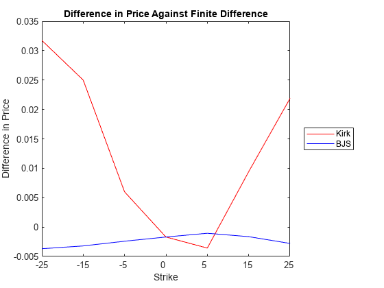
The difference in prices between the closed form and finite difference method is plotted below. It is clear that as the strike moves further away from 0, the difference between the Kirk's approximation and finite difference (red line) increases, while the difference between the Bjerksund and Stensland model and finite difference (blue line) stays at the same level. As stated in [3], the Kirk's approximation is overpricing the spread option when the strike is far away from 0.

% Plot of difference in price against the benchmark
figure;
plot(PriceKirk-PriceFD, 'Color', 'red');
hold on;
plot(PriceBJS-PriceFD, 'Color', 'blue');
hold off;
title('Difference in Price Against Finite Difference');
legend('Kirk', 'BJS', 'Location', 'EastOutside');
xlabel('Strike');
ax = gca;
ax.XTickLabel = Strike;
ylabel('Difference in Price');

Figure contains an axes object. The axes object with title Difference in Price Against Finite Difference, xlabel Strike, ylabel Difference in Price contains 2 objects of type line. These objects represent Kirk, BJS.

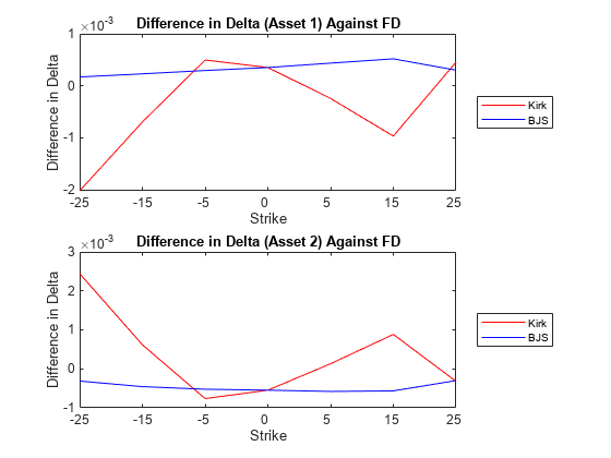
Next, the difference in delta between the closed form models and finite difference is plotted. The top plot shows the difference in delta for the first asset, and the bottom plot shows the difference in delta for the second asset. As seen from the small increments in the y-axis of the order 10e-3, it can be seen that all three models (Kirk, BJS, finite difference) produce similar values for delta.

% Plot of difference in delta of first asset against the benchmark
figure;
subplot(2, 1, 1);
plot(DeltaKirk(:,1)-DeltaFD(:,1), 'Color', 'red');
hold on;
plot(DeltaBJS(:,1)-DeltaFD(:,1), 'Color', 'blue');
hold off;
title('Difference in Delta (Asset 1) Against FD');
legend('Kirk', 'BJS', 'Location', 'EastOutside');
xlabel('Strike');
ax = gca;
ax.XTickLabel = Strike;
ylabel('Difference in Delta');

% Plot of difference in delta of second asset against the benchmark
subplot(2, 1, 2);
plot(DeltaKirk(:,2)-DeltaFD(:,2), 'Color', 'red');
hold on;
plot(DeltaBJS(:,2)-DeltaFD(:,2), 'Color', 'blue');
hold off;
title('Difference in Delta (Asset 2) Against FD');
legend('Kirk', 'BJS', 'Location', 'EastOutside');
xlabel('Strike');
ax = gca;
ax.XTickLabel = Strike;
ylabel('Difference in Delta');

Figure contains 2 axes objects. Axes object 1 with title Difference in Delta (Asset 1) Against FD, xlabel Strike, ylabel Difference in Delta contains 2 objects of type line. These objects represent Kirk, BJS. Axes object 2 with title Difference in Delta (Asset 2) Against FD, xlabel Strike, ylabel Difference in Delta contains 2 objects of type line. These objects represent Kirk, BJS.

Analyzing Prices and Vega at Different Levels of Volatility

To further show the type of analysis that can be conducted using these models, the above spread option is priced at different levels of volatility for the first asset. The price and vega are compared at three levels of volatility for the first asset: 0.1, 0.3, and 0.5. The Bjerksund and Stensland model is used for this analysis.

% Strike
Strike = 5;

% Specify output
OutSpec = {'Price', 'Vega'};

% Different levels of volatility for asset 1
Vol1 = [0.1, 0.3, 0.5];

StockSpec1 = stockspec(Vol1, Price1, 'Continuous', Div1);

% Bjerksund and Stensland model
[PriceBJS, VegaBJS] = ...
    spreadsensbybjs(RateSpec, StockSpec1, StockSpec2, Settle, ...
    Maturity, OptSpec, Strike, Corr, 'OutSpec', OutSpec);

displaySummary(Vol1, PriceBJS, VegaBJS)

Prices for different vol levels in asset 1:

8.366158
14.209112
21.795746

Asset 1 vega for different vol levels in asset 1:

15.534849
36.212192
38.794348

Asset 2 vega for different vol levels in asset 1:

29.437036
7.133657
-0.557852

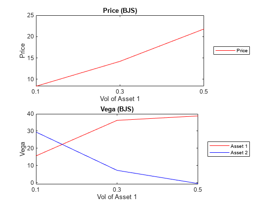
The change in the price and vega with respect to the volatility of the first asset is plotted below. You can observe that as the volatility of the first asset increases, the price of the spread option also increases. Also, the changes in vega indicate that the price of the spread option becomes more sensitive to the volatility of the first asset and less sensitive to the volatility of the second asset.

figure;

% Plot price for BJS model
subplot(2, 1, 1);
plot(PriceBJS, 'Color', 'red');
title('Price (BJS)');
legend('Price', 'Location', 'EastOutside');
xlabel('Vol of Asset 1');
ax = gca;
ax.XTick = 1:3;
ax.XTickLabel = Vol1;
ylabel('Price');

% Plot of vega for BJS model
subplot(2, 1, 2);
plot(VegaBJS(:,1), 'Color', 'red');
hold on;
plot(VegaBJS(:,2), 'Color', 'blue');
hold off;
title('Vega (BJS)');
legend('Asset 1', 'Asset 2', 'Location', 'EastOutside');
xlabel('Vol of Asset 1');
ax = gca;
ax.XTick = 1:3;
ax.XTickLabel = Vol1;
ax.YLim = [-1 40];
ylabel('Vega');

Figure contains 2 axes objects. Axes object 1 with title Price (BJS), xlabel Vol of Asset 1, ylabel Price contains an object of type line. This object represents Price. Axes object 2 with title Vega (BJS), xlabel Vol of Asset 1, ylabel Vega contains 2 objects of type line. These objects represent Asset 1, Asset 2.

Summary

In this example, European and American spread options are priced and analyzed using various techniques. The Financial Instruments Toolbox™ provides functions for two types of closed form solutions (Kirk, BJS), the finite difference method, and the Monte Carlo simulation method. The closed form solutions are well suited for pricing and sensitivity calculation of European spread options because they are fast. However, they cannot price American spread options. The finite difference method and Monte Carlo method can price both European and American options. However, they are not as fast in pricing European spread options as compared to closed form solutions.

References

[1] Carmona, Rene, Durrleman, Valdo. "Pricing and Hedging Spread Options." SIAM Review. Vol. 45, No. 4, 2003, pp. 627-685.

[2] Wilmott, Paul, Dewynne, Jeff, Howison, Sam. Option Pricing. Oxford Financial Press, 1993.

[3] Bjerksund, Petter, Stensland, Gunnar. "Closed form spread option valuation." Department of Finance, NHH, 2006.

[4] Longstaff, Francis A, Schwartz, Eduardo S. "Valuing American Options by Simulation: A Simple Least-Squares Approach." Anderson Graduate School of Management, UC Los Angeles, 2001.

Utility Functions

function displayComparison(model1, model2, price1, price2, delta1, delta2, gamma1, gamma2)
% Pad the model name with additional spaces
additionalSpaces = numel(model1) - numel(model2);
if additionalSpaces > 0
    model2 = [model2 repmat(' ', 1, additionalSpaces)];
else
    model1 = [model1 repmat(' ', 1, abs(additionalSpaces))];
end
    
% Comparison of calculated prices
fprintf('Comparison of prices:\n');
fprintf('\n');
fprintf('%s:   % f\n', model1, price1);
fprintf('%s:   % f\n', model2, price2);
fprintf('\n');

% Comparison of Delta
fprintf('Comparison of delta:\n');
fprintf('\n');
fprintf('%s:   % f     % f\n', model1, delta1(1), delta1(2));
fprintf('%s:   % f     % f\n', model2, delta2(1), delta2(2));
fprintf('\n');

% Comparison of Gamma
fprintf('Comparison of gamma:\n');
fprintf('\n');
fprintf('%s:   % f     % f\n', model1, gamma1(1), gamma1(2));
fprintf('%s:   % f     % f\n', model2, gamma2(1), gamma2(2));
fprintf('\n');
end

function displayComparisonPrices(PriceKirk, PriceBJS, PriceFD, Strike)
% Comparison of calculated prices
fprintf('Prices for range of strikes:\n');
fprintf('\n')
fprintf('Kirk     \tBJS      \tFD    \n');
for i = 1:numel(Strike)
    fprintf('%f\t%f\t%f\n', PriceKirk(i), PriceBJS(i), PriceFD(i));
end
end

function displaySummary(Vol1, PriceBJS, VegaBJS)
% Display price
fprintf('Prices for different vol levels in asset 1:\n');
fprintf('\n');
for i = 1:numel(Vol1)
    fprintf('%f\n', PriceBJS(i));
end
fprintf('\n');

% Display vega for first asset
fprintf('Asset 1 vega for different vol levels in asset 1:\n');
fprintf('\n');
for i = 1:numel(Vol1)
    fprintf('%f\n', VegaBJS(i,1));
end
fprintf('\n');

% Display vega for second asset
fprintf('Asset 2 vega for different vol levels in asset 1:\n');
fprintf('\n');
for i = 1:numel(Vol1)
    fprintf('%f\n', VegaBJS(i,2));
end
end