spreadbyfd

Price European or American spread options using finite difference method

Syntax

Price = spreadbyfd(RateSpec,StockSpec1,StockSpec2,Settle,Maturity,OptSpec,Strike,Corr)

Price = spreadbyfd(___,Name,Value)

[Price,PriceGrid,AssetPrice1,AssetPrice2,Times]
= spreadbyfd(RateSpec,StockSpec1,StockSpec2,Settle,Maturity,OptSpec,Strike,Corr)

[Price,PriceGrid,AssetPrice1,AssetPrice2,Times]
= spreadbyfd(___,Name,Value)

Description

Price = spreadbyfd(RateSpec,StockSpec1,StockSpec2,Settle,Maturity,OptSpec,Strike,Corr) returns the price of European or American call or put spread options using the Alternate Direction Implicit (ADI) finite difference method. The spread is between the asset defined in StockSpec1 minus the asset defined in StockSpec2.

example

Price = spreadbyfd(___,Name,Value) adds optional name-value pair arguments.

[Price,PriceGrid,AssetPrice1,AssetPrice2,Times] = spreadbyfd(RateSpec,StockSpec1,StockSpec2,Settle,Maturity,OptSpec,Strike,Corr) returns the Price, PriceGrid, AssetPrice1, AssetPrice2, and Times for a European or American call or put spread options using the Alternate Direction Implicit (ADI) finite difference method. The spread is between the asset defined in StockSpec1 minus the asset defined in StockSpec2.

[Price,PriceGrid,AssetPrice1,AssetPrice2,Times] = spreadbyfd(___,Name,Value) returns the Price, PriceGrid, AssetPrice1, AssetPrice2, and Times and adds optional name-value pair arguments.

Examples

collapse all

Compute the Price of a Spread Option Using the Alternate Direction Implicit (ADI) Finite Difference Method

Open Live Script

Define the spread option dates.

Settle = datetime(2012,1,1);
Maturity = datetime(2012,4,1);

Define asset 1. Price and volatility of RBOB gasoline

  Price1gallon = 2.85;          % $/gallon
  Price1 = Price1gallon * 42;   % $/barrel  
  Vol1 = 0.29;

Define asset 2. Price and volatility of WTI crude oil

  Price2 = 93.20;         % $/barrel
  Vol2 = 0.36;

Define the correlation between the underlying asset prices of asset 1 and asset 2.

Corr = 0.42;

Define the spread option.

OptSpec = 'call';
Strike = 20;

Define the RateSpec.

rates = 0.05;
Compounding = -1;
Basis = 1;
RateSpec = intenvset('ValuationDate', Settle, 'StartDates', Settle, ...
'EndDates', Maturity, 'Rates', rates, ...
'Compounding', Compounding, 'Basis', Basis)

RateSpec = struct with fields:
           FinObj: 'RateSpec'
      Compounding: -1
             Disc: 0.9876
            Rates: 0.0500
         EndTimes: 0.2500
       StartTimes: 0
         EndDates: 734960
       StartDates: 734869
    ValuationDate: 734869
            Basis: 1
     EndMonthRule: 1

Define the StockSpec for the two assets.

StockSpec1 = stockspec(Vol1, Price1)

StockSpec1 = struct with fields:
             FinObj: 'StockSpec'
              Sigma: 0.2900
         AssetPrice: 119.7000
       DividendType: []
    DividendAmounts: 0
    ExDividendDates: []

StockSpec2 = stockspec(Vol2, Price2)

StockSpec2 = struct with fields:
             FinObj: 'StockSpec'
              Sigma: 0.3600
         AssetPrice: 93.2000
       DividendType: []
    DividendAmounts: 0
    ExDividendDates: []

Compute the spread option price based on the Alternate Direction Implicit (ADI) finite difference method.

[Price, PriceGrid, AssetPrice1, AssetPrice2, Times] = ...
 spreadbyfd(RateSpec, StockSpec1, StockSpec2, Settle, ...
 Maturity, OptSpec, Strike, Corr);

Display the price.

Price

Price = 
11.1998

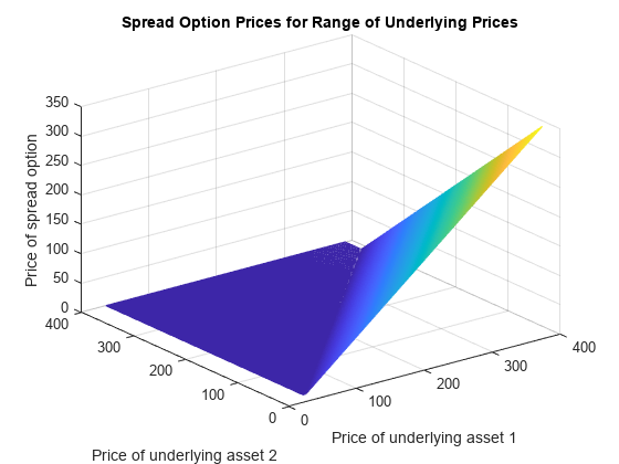
Plot the finite difference grid.

mesh(AssetPrice1, AssetPrice2, PriceGrid(:, :, 1)');
    title('Spread Option Prices for Range of Underlying Prices');
    xlabel('Price of underlying asset 1');
    ylabel('Price of underlying asset 2');
    zlabel('Price of spread option');

Figure contains an axes object. The axes object with title Spread Option Prices for Range of Underlying Prices, xlabel Price of underlying asset 1, ylabel Price of underlying asset 2 contains an object of type surface.

Input Arguments

collapse all

`RateSpec` — Interest-rate term structure
structure

Interest-rate term structure (annualized and continuously compounded), specified by the RateSpec obtained from intenvset. For information on the interest-rate specification, see intenvset.

Data Types: struct

`StockSpec1` — Stock specification for underlying asset 1
structure

Stock specification for underlying asset 1. For information on the stock specification, see stockspec.

stockspec can handle other types of underlying assets. For example, for physical commodities the price is represented by StockSpec.Asset, the volatility is represented by StockSpec.Sigma, and the convenience yield is represented by StockSpec.DividendAmounts.

Data Types: struct

`StockSpec2` — Stock specification for underlying asset 2
structure

Stock specification for underlying asset 2. For information on the stock specification, see stockspec.

Data Types: struct

`Settle` — Settlement dates for spread option
datetime array | string array | date character vector

Settlement dates for the spread option, specified as a NINST-by-1 vector using a datetime array, string array, or date character vectors.

To support existing code, spreadbyfd also accepts serial date numbers as inputs, but they are not recommended.

`Maturity` — Maturity date for spread option
datetime array | string array | date character vector

Maturity date for spread option, specified as a NINST-by-1 vector using a datetime array, string array, or date character vectors.

To support existing code, spreadbyfd also accepts serial date numbers as inputs, but they are not recommended.

`OptSpec` — Definition of option
character vector with values `'call'` or `'put'` | cell array of character vectors

Definition of option as 'call' or 'put', specified as a NINST-by-1 cell array of character vectors.

Data Types: char | cell

`Strike` — Option strike price values
integer | vector of integers

Option strike price values, specified as an integer using a NINST-by-1 vector of strike price values.

Data Types: double

`Corr` — Correlation between underlying asset prices
integer | vector of integers

Correlation between underlying asset prices, specified as an integer using a NINST-by-1 vector.

Data Types: double

Name-Value Arguments

Specify optional pairs of arguments as Name1=Value1,...,NameN=ValueN, where Name is the argument name and Value is the corresponding value. Name-value arguments must appear after other arguments, but the order of the pairs does not matter.

Before R2021a, use commas to separate each name and value, and enclose Name in quotes.

Example: [Price,PriceGrid,AssetPrice1,AssetPrice2,Times] = spreadbyfd(RateSpec,StockSpec1,StockSpec2,Settle,Maturity,OptSpec,Strike,Corr,'AssetPriceMin','AssetPriceMax','PriceGridSize','TimeGridSize','AmericanOpt',0)

`AssetPriceMin` — Minimum price for price grid boundary
if unspecified, `StockSpec` values are calculated based on asset distributions at maturity (default) | array

Minimum price for price grid boundary, specified as the comma-separated pair consisting of 'AssetPriceMin' and a 1-by-2 array. The first entry in the array corresponds to the first asset defined by StockSpec1 and the second entry corresponds to the second asset defined by StockSpec2.

For the finite difference method, the composition of the grid affects the quality of the output and the execution time. It is highly recommended to use the optional arguments AssetPriceMin, AssetPriceMax, PriceGridSize, and TimeGridSize to control the composition of the grid to ensure the quality of the output and a reasonable execution time.

References

[1] Carmona, R., Durrleman, V. “Pricing and Hedging Spread Options.” SIAM Review. Vol. 45, No. 4, pp. 627–685, Society for Industrial and Applied Mathematics, 2003.
[2] Villeneuve, S., Zanette, A. “Parabolic ADI Methods for Pricing American Options on Two Stocks.” Mathematics of Operations Research. Vol. 27, No. 1, pp. 121–149, INFORMS, 2002.
[3] Ikonen, S., Toivanen, J. Efficient Numerical Methods for Pricing American Options Under Stochastic Volatility. Wiley InterScience, 2007.
Version History
Introduced in R2013b