fixed.qrMatrixSolve
Solve system of linear equations Ax = B for x using QR decomposition
Syntax
Description
x = fixed.qrMatrixSolve(A,B, outputType)outputType.
x = fixed.qrMatrixSolve(A,B,outputType,regularizationParameter)
where A is an m-by-n matrix, B is an m-by-p matrix, and λ is the regularization parameter.
Examples
This example shows how to solve a simple system of linear equations , using QR decomposition.
In this example, define A as a 5-by-3 matrix with a large condition number. To solve a system of linear equations involving ill-conditioned (large condition number) non-square matrices, you must use QR decomposition.
rng default;
A = gallery('randsvd', [5,3], 1000000);
b = [1; 1; 1; 1; 1];
x = fixed.qrMatrixSolve(A,b)
x = 3×1
104 ×

   -2.3777
    7.0686
   -2.2703
Compare the result of the fixed.qrMatrixSolve function with the result of the mldivide or \ function.
x = A\b
x = 3×1
104 ×

   -2.3777
    7.0686
   -2.2703
This example shows the effect of a regularization parameter when solving an overdetermined system. In this example, a quantity y is measured at several different values of time t to produce the following observations.
t = [0 .3 .8 1.1 1.6 2.3]';
y = [.82 .72 .63 .60 .55 .50]';
Model the data with a decaying exponential function
.
The preceding equation says that the vector y should be approximated by a linear combination of two other vectors. One is a constant vector containing all ones and the other is the vector with components exp(-t). The unknown coefficients, and , can be computed by doing a least-squares fit, which minimizes the sum of the squares of the deviations of the data from the model. There are six equations and two unknowns, represented by a 6-by-2 matrix.
E = [ones(size(t)) exp(-t)]
E = 6×2

    1.0000    1.0000
    1.0000    0.7408
    1.0000    0.4493
    1.0000    0.3329
    1.0000    0.2019
    1.0000    0.1003
Use the fixed.qrMatrixSolve function to get the least-squares solution.
c = fixed.qrMatrixSolve(E, y)
c = 2×1

    0.4760
    0.3413
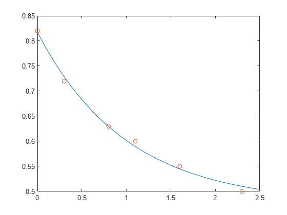
In other words, the least-squares fit to the data is
The following statements evaluate the model at regularly spaced increments in t, and then plot the result together with the original data:
T = (0:0.1:2.5)';
Y = [ones(size(T)) exp(-T)]*c;
plot(T,Y,'-',t,y,'o')
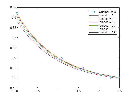
In cases where the input matrices are ill-conditioned, small positive values of a regularization parameter can improve the conditioning of the least squares problem, and reduce the variance of the estimates. Explore the effect of the regularization parameter on the least squares solution for this data.
figure;
lambda = [0:0.1:0.5];
plot(t,y,'o', 'DisplayName', 'Original Data');
for i = 1:length(lambda)
 c = fixed.qrMatrixSolve(E, y, numerictype('double'), lambda(i));
 Y = [ones(size(T)) exp(-T)]*c;
 hold on
 plot(T,Y,'-', 'DisplayName', ['lambda =', num2str(lambda(i))])
end
legend('Original Data', 'lambda = 0', 'lambda = 0.1', 'lambda = 0.2', 'lambda = 0.3', 'lambda = 0.4', 'lambda = 0.5')
Input Arguments
Output Arguments
Extended Capabilities
Version History
Introduced in R2020b
See Also
fixed.backwardSubstitute | fixed.forwardSubstitute | fixed.qlessQR | fixed.qlessQRUpdate | fixed.qrAB | fixed.qlessQRMatrixSolve
Topics
- Algorithms to Determine Fixed-Point Types for Complex Least-Squares Matrix Solve AX=B
- Determine Fixed-Point Types for Complex Least-Squares Matrix Solve AX=B
- Algorithms to Determine Fixed-Point Types for Real Least-Squares Matrix Solve AX=B
- Determine Fixed-Point Types for Real Least-Squares Matrix Solve AX=B