Main Content

ggiwphd

Gamma Gaussian Inverse Wishart (GGIW) PHD filter

Description

The ggiwphd object is a filter that implements the probability hypothesis density (PHD) using a mixture of Gamma Gaussian Inverse-Wishart components.

GGIW implementation of a PHD filter is typically used to track extended objects. An extended object can produce multiple detections per sensor, and the GGIW filter uses the random matrix model to account for the spatial distribution of these detections. The filter consists of three distributions to represent the state of an extended object.

  1. Gaussian distribution — represents the kinematic state of the extended object.

  2. Gamma distribution — represents the expected number of detections on a sensor from the extended object.

  3. Inverse-Wishart (IW) distribution — represents the spatial extent of the target. In 2-D space, the extent is represented by a 2-by-2 random positive definite matrix, which corresponds to a 2-D ellipse description. In 3-D space, the extent is represented by a 3-by-3 random matrix, which corresponds to a 3-D ellipsoid description. The probability density of these random matrices is given as an Inverse-Wishart distribution.

For details about ggiwphd, see [1] and [2].

Note

ggiwphd object is not compatible with trackerGNN, trackerJPDA, and trackerTOMHT system objects.

Creation

Description

PHD = ggiwphd creates a ggiwphd filter with default property values.

PHD = ggiwphd(States,StateCovariances) allows you to specify the States and StateCovariances of the Gaussian distribution for each component in the density. States and StateCovariances set the properties of the same names.

example

phd = ggiwphd(States,StateCovariances,Name,Value) also allows you to set properties for the filter using one or more name-value pairs. Enclose each property name in quotes.

Properties

expand all

State of each component in the filter, specified as a P-by-N matrix, where P is the dimension of the state and N is the number of components. Each column of the matrix corresponds to the state of each component. The default value for States is a 6-by-2 matrix, in which the elements of the first column are all 0, and the elements of the second column are all 1.

If you want a filter with single-precision floating-point variables, specify States as single-precision vector variables. For example,

filter = ggiwphd(single(zeros(6,4)),single(ones(6,6,4)))

Data Types: single | double

State estimate error covariance of each component in the filter, specified as a P-by-P-by-N array, where P is the dimension of the state and N is the number of components. Each page (P-by-P matrix) of the array corresponds to the covariance matrix of each component. The default value for StateCovariances is a 6-by-6-by-2 array, in which each page (6-by-6 matrix) is an identity matrix.

Data Types: single | double

Indices of position coordinates in the state, specified as a row vector of positive integers. For example, by default the state is arranged as [x;vx;y;vy;z;vz] and the corresponding position index is [1 3 5] representing x-, y- and z-position coordinates.

Example: [1 2 3]

Data Types: single | double

State transition function, specified as a function handle. This function calculates the state vector at time step k from the state vector at time step k–1. The function can also include noise values.

  • If HasAdditiveProcessNoise is true, specify the function using one of these syntaxes:

    x(k) = transitionfcn(x(k-1))
    
    x(k) = transitionfcn(x(k-1),dT)
    where x(k) is the state estimate at time k, and dT is the time step.

  • If HasAdditiveProcessNoise is false, specify the function using one of these syntaxes:

    x(k) = transitionfcn(x(k-1),w(k-1))
    
    x(k) = transitionfcn(x(k-1),w(k-1),dT)
    where x(k) is the state estimate at time k, w(k) is the process noise at time k, and dT is the time step.

Example: @constacc

Data Types: function_handle

The Jacobian of the state transition function, specified as a function handle. This function has the same input arguments as the state transition function.

  • If HasAdditiveProcessNoise is true, specify the Jacobian function using one of these syntaxes:

    Jx(k) = statejacobianfcn(x(k))
    
    Jx(k) = statejacobianfcn(x(k),dT)
    where x(k) is the state at time k, dT is the time step, and Jx(k) denotes the Jacobian of the state transition function with respect to the state. The Jacobian is an M-by-M matrix at time k, where M is the dimension of the state.

  • If HasAdditiveProcessNoise is false, specify the Jacobian function using one of these syntaxes:

    [Jx(k),Jw(k)] = statejacobianfcn(x(k),w(k))
    
    [Jx(k),Jw(k)] = statejacobianfcn(x(k),w(k),dT)
    where w(k) is a Q-element vector of the process noise at time k. Q is the dimension of the process noise. Unlike the case of additive process noise, the process noise vector in the nonadditive noise case need not have the same dimensions as the state vector.

    Jw(k) denotes the M-by-Q Jacobian of the predicted state with respect to the process noise elements, where M is the dimension of the state.

If not specified, the Jacobians are computed by numerical differencing at each call of the predict function. This computation can increase the processing time and numerical inaccuracy.

Example: @constaccjac

Data Types: function_handle

Process noise covariance:

  • When HasAdditiveProcessNoise is true, specify the process noise covariance as a scalar or a positive definite real-valued M-by-M matrix. M is the dimension of the state vector. When specified as a scalar, the matrix is a multiple of the M-by-M identity matrix.

  • When HasAdditiveProcessNoise is false, specify the process noise covariance as a Q-by-Q matrix. Q is the size of the process noise vector. You must specify ProcessNoise before any call to the predict object function.

Example: [1.0 0.05; 0.05 2]

Option to model processes noise as additive, specified as true or false. When this property is true, process noise is added to the state vector. Otherwise, noise is incorporated into the state transition function.

Example: true

Shape parameter of Gamma distribution for each component, specified as a 1-by-N row vector of positive real values. N is the number of components in the density.

Example: [1.0 0.95 2]

Data Types: single | double

Rate parameter of Gamma distribution for each component, specified as a 1-by-N row vector of positive real values. N is the number of components in the density.

Example: [1.2 0.85 1.5]

Data Types: single | double

Forgetting factor of Gamma distribution for each component, specified as a 1-by-N row vector of positive real values. N is the number of components in the density. During prediction, for each component, the Gamma distribution parameters, shape (α) and rate (β), are both divided by forgetting factor n:

ak+1||k=αknkβk+1|k=βknk

where k and k+1 represent two consecutive time steps. The mean (E) and variance (Var) of a Gamma distribution are:

E=αβVar=αβ2

Therefore, the division action will keep the expected measurement rate as a constant, but increase the variance of the Gamma distribution exponentially with time if the forgetting factor n is larger than 1.

Example: [1.2 1.1 1.4]

Data Types: single | double

Degrees of freedom parameter of Inverse-Wishart distribution for each component, specified as a 1-by-N row vector of positive real values. N is the number of components in the density.

Example: [55.2 31.1 20.4]

Data Types: single | double

Scale matrix of Inverse-Wishart distribution for each component, specified as a d-by-d-by-N array of positive real values. d is the dimension of the space (for example, d = 2 for 2-D space), and N is the number of components in the density. The default value for ScaleMatrices is a 3-by-3-by-2 array, where each page (3-by-3 matrix) of the array is 100*eye(3).

Example: 20*eye(3,3,4)

Data Types: single | double

Rotation transition function of target's extent, specified as a function handle. The function allows predicting the rotation of the target's extent when the object's angular velocity is estimated in the state vector. To define your own extent rotation function, follow the syntax given by

R = myRotationFcn(x,dT)

where x is the component state, dT is the time step, and R is the corresponding rotation matrix. Note that R is returned as a 2-by-2 matrix if the extent is 2-D, and a 3-by-3 matrix if the extent is 3-D. The extent at the next step is given by

Ex(t+dT)=R×Ex(t)×RT

where Ex(t) is the extent at time t.

Example: @myRotationFcn

Data Types: function_handle

Temporal decay factor of IW distribution, specified as a positive scalar. You can use this property to control the extent uncertainty (variance of IW distribution) during prediction. The smaller the TemporalDecay value is, the faster the variance of IW distribution increases.

Example: 120

Data Types: single | double

Label of each component in the mixture, specified as a 1-by-N row vector of nonnegative integers. N is the number of components in the density. Each component can only have one label, but multiple components can share the same label.

Example: [1 2 3]

Data Types: single | double

Weight of each component in the density, specified as a 1-by-N row vector of positive real values. N is the number of components in the density. The weights are given in the sequence as shown in the labels property.

Example: [1.1 0.82 1.1]

Data Types: single | double

Detections, specified as a K-element cell array of objectDetection objects, where K is the number of detections. You can create detections directly, or you can obtain detections from the outputs of sensor objects, such as radarSensor, monostaticRadarSensor, irSensor, and sonarSensor.

Data Types: single | double

Measurement model function, specified as a function handle. This function specifies the transition from state to measurement. Input to the function is the P-element state vector. The output is the M-element measurement vector. The function can take additional input arguments, such as sensor position and orientation.

  • If HasAdditiveMeasurementNoise is true, specify the function using one of these syntaxes:

    z(k) = measurementfcn(x(k))
    
    z(k) = measurementfcn(x(k),parameters)
    where x(k) is the state at time k and z(k) is the corresponding measurement. The parameters argument stands for all additional arguments required by the measurement function.

  • If HasAdditiveMeasurementNoise is false, specify the function using one of these syntaxes:

    z(k) = measurementfcn(x(k),v(k))
    
    z(k) = measurementfcn(x(k),v(k),parameters)
    where x(k) is the state at time k and v(k) is the measurement noise at time k. The parameters argument stands for all additional arguments required by the measurement function.

Example: @cameas

Data Types: function_handle

Jacobian of the measurement function, specified as a function handle. The function has the same input arguments as the measurement function. The function can take additional input parameters, such as sensor position and orientation.

  • If HasAdditiveMeasurmentNoise is true, specify the Jacobian function using one of these syntaxes:

    Jmx(k) = measjacobianfcn(x(k))
    
    Jmx(k) = measjacobianfcn(x(k),parameters)
    where x(k) is the state at time k. Jmx(k) denotes the M-by-P Jacobian of the measurement function with respect to the state. M is the dimension of the measurement, and P is the dimension of the state. The parameters argument stands for all arguments required by the measurement function.

  • If HasAdditiveMeasurmentNoise is false, specify the Jacobian function using one of these syntaxes:

    [Jmx(k),Jmv(k)] = measjacobianfcn(x(k),v(k))
    
    [Jmx(k),Jmv(k)] = measjacobianfcn(x(k),v(k),parameters)
    where x(k) is the state at time k and v(k) is an R-dimensional sample noise vector. Jmx(k) denotes the M-by-P Jacobian matrix of the measurement function with respect to the state. Jmv(k) denotes the Jacobian of the M-by-R measurement function with respect to the measurement noise. The parameters argument stands for all arguments required by the measurement function.

If not specified, measurement Jacobians are computed using numerical differencing at each call to the correct function. This computation can increase processing time and numerical inaccuracy.

Example: @cameasjac

Data Types: function_handle

Option to model measurement noise as additive, specified as true or false. When this property is true, measurement noise is added to the state vector. Otherwise, noise is incorporated into the measurement function.

Example: true

Maximum number of detections the ggiwphd filter can take as input, specified as a positive integer.

Example: 50

Data Types: single | double

Maximum number of components the ggiwphd filter can maintain, specified as a positive integer.

Note

When you use a ggiwphd object in a trackerPHD object by specifying the SensorConfigurations property of the tracker, the tracker determines the maximum number of components based on its own MaxNumComponents property instead of the MaxNumComponents property of the ggiwphd object.

Data Types: single | double

Object Functions

appendAppend two phd filter objects
correctCorrect phd filter with detections
correctUndetectedCorrect phd filter with no detection hypothesis
extractStateExtract target state estimates from the phd filter
labeledDensityKeep components with a given label ID
likelihoodLog-likelihood of association between detection cells and components in the density
mergeMerge components in the density of phd filter
predictPredict probability hypothesis density of phd filter
prunePrune the filter by removing selected components
scaleScale weights of components in the density
cloneCreate duplicate phd filter object

Examples

collapse all

Creating a ggiwphd filter with two 3-D constant velocity components. The initial states of the two components are [0;0;0;0;0;0] and [1;0;1;0;1;0], respectively. Both these components have position covariance equal to 1 and velocity covariance equal to 100. By default, ggiwphd creates a 3-D extent matrix for each component.

states = [zeros(6,1),[1;0;1;0;1;0]];
cov1 = diag([1 100 1 100 1 100]);
covariances = cat(3,cov1,cov1);

phd = ggiwphd(states,covariances,'StateTransitionFcn',@constvel,...
             'StateTransitionJacobianFcn',@constveljac,...
             'MeasurementFcn',@cvmeas,'MeasurementJacobianFcn',@cvmeasjac,...
             'ProcessNoise',eye(3),'HasAdditiveProcessNoise',false,...
             'PositionIndex',[1;3;5]);

Specify information about extent.

dofs = [21 30];
scaleMatrix1 = 13*diag([4.7 1.8 1.4].^2);
scaleMatrix2 = 22*diag([1.8 4.7 1.4].^2); 
scaleMatrices = cat(3,scaleMatrix1,scaleMatrix2);
phd.DegreesOfFreedom = dofs;
phd.ScaleMatrices = scaleMatrices;
phd.ExtentRotationFcn = @(x,dT)eye(3); % No rotation during prediction

Predict the filter 0.1 second ahead.

predict(phd,0.1);

Specify detections at 0.1 second. The filter receives 10 detections at the current scan.

detections = cell(10,1);
rng(2018); % Reproducible results
for i = 1:10
   detections{i} = objectDetection(0.1,randi([0 1]) + randn(3,1));
end
phd.Detections = detections;

Select two detection cells and calculate their likelihoods.

detectionIDs = false(10,2);
detectionIDs([1 3 5 7 9],1) = true;
detectionIDs([2 4 6 8 10],2) = true;
lhood = likelihood(phd,detectionIDs)
lhood = 2×2

    1.5575   -0.3183
    0.1513   -0.7616

Correct the filter with the two detection cells and associated likelihoods.

correct(phd,detectionIDs, exp(lhood)./sum(exp(lhood),1));
phd
phd = 
  ggiwphd with properties:

                         States: [6x4 double]
               StateCovariances: [6x6x4 double]
                  PositionIndex: [3x1 double]
             StateTransitionFcn: @constvel
     StateTransitionJacobianFcn: @constveljac
                   ProcessNoise: [3x3 double]
        HasAdditiveProcessNoise: 0

                         Shapes: [6 6 6 6]
                          Rates: [2 2 2 2]
         GammaForgettingFactors: [1 1 1 1]

               DegreesOfFreedom: [25.9870 34.9780 25.9870 34.9780]
                  ScaleMatrices: [3x3x4 double]
              ExtentRotationFcn: @(x,dT)eye(3)
                  TemporalDecay: 100

                        Weights: [0.8032 0.1968 0.6090 0.3910]
                         Labels: [0 0 0 0]

                     Detections: {1x10 cell}
                 MeasurementFcn: @cvmeas
         MeasurementJacobianFcn: @cvmeasjac
    HasAdditiveMeasurementNoise: 1

Merge components in the filter.

merge(phd,5);
phd
phd = 
  ggiwphd with properties:

                         States: [6x2 double]
               StateCovariances: [6x6x2 double]
                  PositionIndex: [3x1 double]
             StateTransitionFcn: @constvel
     StateTransitionJacobianFcn: @constveljac
                   ProcessNoise: [3x3 double]
        HasAdditiveProcessNoise: 0

                         Shapes: [6 6.0000]
                          Rates: [2 2]
         GammaForgettingFactors: [1 1]

               DegreesOfFreedom: [25.9870 34.9780]
                  ScaleMatrices: [3x3x2 double]
              ExtentRotationFcn: @(x,dT)eye(3)
                  TemporalDecay: 100

                        Weights: [1.4122 0.5878]
                         Labels: [0 0]

                     Detections: {1x10 cell}
                 MeasurementFcn: @cvmeas
         MeasurementJacobianFcn: @cvmeasjac
    HasAdditiveMeasurementNoise: 1

Extract state estimates and detections.

targetStates = extractState(phd,0.5);
tStates = targetStates.State
tStates = 6×1

    0.1947
    0.9733
    0.8319
    4.1599
   -0.0124
   -0.0621

    
d = [detections{:}];
measurements = [d.Measurement];

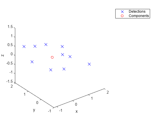
Visualize the results.

figure()
plot3(measurements(1,:),measurements(2,:),measurements(3,:),'x','MarkerSize',10,'MarkerEdgeColor','b');
hold on;
plot3( tStates(1,:),tStates(3,:),tStates(5,:),'ro');
xlabel('x')
ylabel('y')
zlabel('z')
legend('Detections','Components')

References

[1] Granstorm, K., and O. Orguner." A PHD filter for tracking multiple extended targets using random matrices." IEEE Transactions on Signal Processing. Vol. 60, Number 11, 2012, pp. 5657-5671.

[2] Granstorm, K., and A. Natale, P. Braca, G. Ludeno, and F. Serafino."Gamma Gaussian inverse Wishart probability hypothesis density for extended target tracking using X-band marine radar data." IEEE Transactions on Geoscience and Remote Sensing. Vol. 53, Number 12, 2015, pp. 6617-6631.

Extended Capabilities

Version History

Introduced in R2019a