gpsSensor
GPS receiver simulation model
Description
The gpsSensor
System object™ models data output from a Global Positioning System (GPS) receiver. The object
models the position noise as a first order Gauss Markov process, in which the sigma values are
specified in the HorizontalPositionAccuracy and the
VerticalPositionAccuracy properties. The object models the velocity
noise as Gaussian noise with its sigma value specified in the
VelocityAccuracy property.
To model a GPS receiver:
Create the
gpsSensorobject and set its properties.Call the object with arguments, as if it were a function.
To learn more about how System objects work, see What Are System Objects?
Creation
Description
GPS = gpsSensorgpsSensor
System object that computes a Global Positioning System receiver reading based on a local
position and velocity input signal. The default reference position in geodetic coordinates is
latitude: 0o N
longitude: 0o E
altitude: 0 m
GPS = gpsSensor('ReferenceFrame',RF)gpsSensor
System object that computes a global positioning system receiver reading relative to the
reference frame RF.
GPS = gpsSensor(___,
sets one or more properties using name-value arguments in addition to any of the previous
input arguments.Name=Value)
Input Arguments
Reference frame of the sensor inputs, specified as either 'NED'
(North-East-Down) or 'ENU' (East-North-Up).
Data Types: char | string
Properties
Unless otherwise indicated, properties are nontunable, which means you cannot change their
values after calling the object. Objects lock when you call them, and the
release function unlocks them.
If a property is tunable, you can change its value at any time.
For more information on changing property values, see System Design in MATLAB Using System Objects.
Update rate of the receiver in Hz, specified as a positive real scalar.
Data Types: single | double
Reference location, specified as a 3-element row vector in geodetic coordinates
(latitude, longitude, and altitude). Altitude is the height above the reference
ellipsoid model, WGS84. The reference location is in [degrees degrees
meters]. The degree format is decimal degrees (DD).
Data Types: single | double
Position coordinate input format, specified as 'Local' or
'Geodetic'.
If you set the property as
'Local', then you need to specify thetruePositioninput as Cartesian coordinates with respect to the local navigation frame whose origin is fixed and defined by theReferenceLcationproperty. Additionally, when you specify thetrueVelocityinput, you need to specify it with respect to this local navigation frame.If you set the property as
'Geodetic', then you need to specify thetruePositioninput as geodetic coordinates in latitude, longitude, and altitude. Additionally, when you specify thetrueVelocityinput, you need to specify it with respect to the navigation frame (NED or ENU) whose origin corresponds to thetruePositioninput. When setting the property as'Geodetic', thegpsSensorobject neglects theReferenceLocationproperty.
Data Types: character vector
Horizontal position accuracy in meters, specified as a nonnegative real scalar. The horizontal position accuracy specifies the standard deviation of the noise in the horizontal position measurement.
Tunable: Yes
Data Types: single | double
Vertical position accuracy in meters, specified as a nonnegative real scalar. The vertical position accuracy specifies the standard deviation of the noise in the vertical position measurement.
Tunable: Yes
Data Types: single | double
Velocity accuracy in meters per second, specified as a nonnegative real scalar. The velocity accuracy specifies the standard deviation of the noise in the velocity measurement.
Tunable: Yes
Data Types: single | double
Global position noise decay factor, specified as a scalar in the range [0,1].
A decay factor of 0 models the global position noise as a white noise process. A decay factor of 1 models the global position noise as a random walk process.
Tunable: Yes
Data Types: single | double
Random number source, specified as a character vector or string:
'Global stream'–– Random numbers are generated using the current global random number stream.'mt19937ar with seed'–– Random numbers are generated using the mt19937ar algorithm with the seed specified by theSeedproperty.
Data Types: char | string
Initial seed of an mt19937ar random number generator algorithm, specified as a nonnegative integer scalar.
Dependencies
To enable this property, set RandomStream to
'mt19937ar with seed'.
Data Types: single | double | int8 | int16 | int32 | int64 | uint8 | uint16 | uint32 | uint64
Usage
Description
[
computes global navigation satellite system receiver readings from the position and
velocity inputs.position,velocity,groundspeed,course] = GPS(truePosition,trueVelocity)
Input Arguments
Position of the GPS receiver in the navigation coordinate system, specified as a real finite N-by-3 matrix. N is the number of samples in the current frame.
When the
PositionInputFormatproperty is specified as'Local', specifytruePositionas Cartesian coordinates with respect to the local navigation frame whose origin is fixed atReferenceLocation.When the
PositionInputFormatproperty is specified as'Geodetic', specifytruePositionas geodetic coordinates in[latitude longitude altitude].latitudeandlongitudeare in degrees.altitudeis the height above the WGS84 ellipsoid model in meters.
Data Types: single | double
Velocity of GPS receiver in the navigation coordinate system in meters per second, specified as a real finite N-by-3 matrix. N is the number of samples in the current frame.
When the
PositionInputFormatproperty is specified as'Local', specifytrueVelocitywith respect to the local navigation frame (NED or ENU) whose origin is fixed atReferenceLocation.When the
PositionInputFormatproperty is specified as'Geodetic', specifytrueVelocitywith respect to the navigation frame (NED or ENU) whose origin corresponds to thetruePositioninput.
Data Types: single | double
Output Arguments
Position of the GPS receiver in the geodetic latitude, longitude, and altitude (LLA) coordinate system, returned as a real finite N-by-3 array. Latitude and longitude are in degrees with North and East being positive. Altitude is in meters.
N is the number of samples in the current frame.
Data Types: single | double
Velocity of the GPS receiver in the local navigation coordinate system in meters per second, returned as a real finite N-by-3 array. N is the number of samples in the current frame.
When the
PositionInputFormatproperty is specified as'Local', the returned velocity is with respect to the local navigation frame whose origin is fixed atReferenceLocation.When the
PositionInputFormatproperty is specified as'Geodetic', the returned velocity is with respect to the navigation frame (NED or ENU) whose origin corresponds to thepositionoutput.
Data Types: single | double
Magnitude of the horizontal velocity of the GPS receiver in the local navigation coordinate system in meters per second, returned as a real finite N-by-1 column vector.
N is the number of samples in the current frame.
Data Types: single | double
Direction of the horizontal velocity of the GPS receiver in the local navigation coordinate system in degrees, returned as a real finite N-by-1 column vector of values between 0 and 360. North corresponds to 360 degrees and East corresponds to 90 degrees.
N is the number of samples in the current frame.
Data Types: single | double
Object Functions
To use an object function, specify the
System object as the first input argument. For
example, to release system resources of a System object named obj, use
this syntax:
release(obj)
Examples
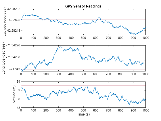
Create a gpsSensor System object™ to model GPS receiver data. Assume a typical one Hz sample rate and a 1000-second simulation time. Define the reference location in terms of latitude, longitude, and altitude (LLA) of Natick, MA (USA). Define the sensor as stationary by specifying the true position and velocity with zeros.
fs = 1;
duration = 1000;
numSamples = duration*fs;

refLoc = [42.2825 -71.343 53.0352];

truePosition = zeros(numSamples,3);
trueVelocity = zeros(numSamples,3);

gps = gpsSensor('SampleRate',fs,'ReferenceLocation',refLoc);
Call gps with the specified truePosition and trueVelocity to simulate receiving GPS data for a stationary platform.
position = gps(truePosition,trueVelocity);
Plot the true position and the GPS sensor readings for position.
t = (0:(numSamples-1))/fs;

subplot(3, 1, 1)
plot(t, position(:,1), ...
     t, ones(numSamples)*refLoc(1))
title('GPS Sensor Readings')
ylabel('Latitude (degrees)')

subplot(3, 1, 2)
plot(t, position(:,2), ...
     t, ones(numSamples)*refLoc(2))
ylabel('Longitude (degrees)')

subplot(3, 1, 3)
plot(t, position(:,3), ...
     t, ones(numSamples)*refLoc(3))
ylabel('Altitude (m)')
xlabel('Time (s)')

The position readings have noise controlled by HorizontalPositionAccuracy, VerticalPositionAccuracy, VelocityAccuracy, and DecayFactor. The DecayFactor property controls the drift in the noise model. By default, DecayFactor is set to 0.999, which approaches a random walk process. To observe the effect of the DecayFactor property:
Reset the
gpsobject.Set
DecayFactorto0.5.Call
gpswith variables specifying a stationary position.Plot the results.
The GPS position readings now oscillate around the true position.
reset(gps)
gps.DecayFactor = 0.5;
position = gps(truePosition,trueVelocity);

subplot(3, 1, 1)
plot(t, position(:,1), ...
     t, ones(numSamples)*refLoc(1))
title('GPS Sensor Readings - Decay Factor = 0.5')
ylabel('Latitude (degrees)')

subplot(3, 1, 2)
plot(t, position(:,2), ...
     t, ones(numSamples)*refLoc(2))
ylabel('Longitude (degrees)')

subplot(3, 1, 3)
plot(t, position(:,3), ...
     t, ones(numSamples)*refLoc(3))
ylabel('Altitude (m)')
xlabel('Time (s)')

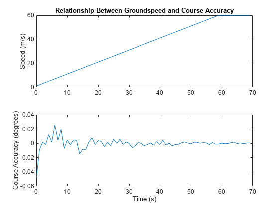
GPS receivers achieve greater course accuracy as groundspeed increases. In this example, you create a GPS receiver simulation object and simulate the data received from a platform that is accelerating from a stationary position.
Create a default gpsSensor System object™ to model data returned by a GPS receiver.
GPS = gpsSensor
GPS =
  gpsSensor with properties:

                    SampleRate: 1                  Hz
           PositionInputFormat: 'Local'
             ReferenceLocation: [0 0 0]            [deg deg m]
    HorizontalPositionAccuracy: 1.6                m
      VerticalPositionAccuracy: 3                  m
              VelocityAccuracy: 0.1                m/s
                  RandomStream: 'Global stream'
                   DecayFactor: 0.999
Create matrices to describe the position and velocity of a platform in the NED coordinate system. The platform begins from a stationary position and accelerates to 60 m/s North-East over 60 seconds, then has a vertical acceleration to 2 m/s over 2 seconds, followed by a 2 m/s rate of climb for another 8 seconds. Assume a constant velocity, such that the velocity is the simple derivative of the position.
duration = 70;
numSamples = duration*GPS.SampleRate;

course = 45*ones(duration,1);
groundspeed = [(1:60)';60*ones(10,1)];

Nvelocity   = groundspeed.*sind(course);
Evelocity   = groundspeed.*cosd(course);
Dvelocity   = [zeros(60,1);-1;-2*ones(9,1)];
NEDvelocity = [Nvelocity,Evelocity,Dvelocity];

Ndistance   = cumsum(Nvelocity);
Edistance   = cumsum(Evelocity);
Ddistance   = cumsum(Dvelocity);
NEDposition = [Ndistance,Edistance,Ddistance];
Model GPS measurement data by calling the GPS object with your velocity and position matrices.
[~,~,groundspeedMeasurement,courseMeasurement] = GPS(NEDposition,NEDvelocity);
Plot the groundspeed and the difference between the true course and the course returned by the GPS simulator.
As groundspeed increases, the accuracy of the course increases. Note that the velocity increase during the last ten seconds has no effect, because the additional velocity is not in the ground plane.
t = (0:numSamples-1)/GPS.SampleRate;

subplot(2,1,1)
plot(t,groundspeed);
ylabel('Speed (m/s)')
title('Relationship Between Groundspeed and Course Accuracy')

subplot(2,1,2)
courseAccuracy = courseMeasurement - course;
plot(t,courseAccuracy)
xlabel('Time (s)');
ylabel('Course Accuracy (degrees)')

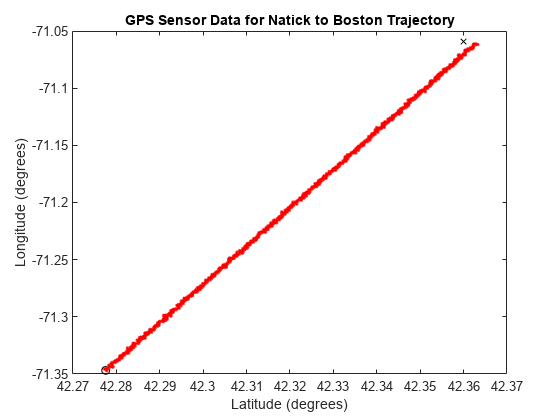
Simulate GPS data received during a trajectory from the city of Natick, MA, to Boston, MA.
Define the decimal degree latitude and longitude for the city of Natick, MA USA, and Boston, MA USA. For simplicity, set the altitude for both locations to zero.
NatickLLA = [42.27752809999999, -71.34680909999997, 0];
BostonLLA = [42.3600825, -71.05888010000001, 0];
Define a motion that can take a platform from Natick to Boston in 20 minutes. Set the origin of the local NED coordinate system as Natick. Create a waypointTrajectory object to output the trajectory 10 samples at a time.
fs = 1;
duration = 60*20;

bearing = 68; % degrees
distance = 25.39e3; % meters
distanceEast = distance*sind(bearing);
distanceNorth = distance*cosd(bearing);

NatickNED = [0,0,0];
BostonNED = [distanceNorth,distanceEast,0];

trajectory = waypointTrajectory( ...
    'Waypoints', [NatickNED;BostonNED], ...
    'TimeOfArrival',[0;duration], ...
    'SamplesPerFrame',10, ...
    'SampleRate',fs);
Create a gpsSensor object to model receiving GPS data for the platform. Set the HorizontalPositionalAccuracy to 25 and the DecayFactor to 0.25 to emphasize the noise. Set the ReferenceLocation to the Natick coordinates in LLA.
GPS = gpsSensor( ...
    'HorizontalPositionAccuracy',25, ...
    'DecayFactor',0.25, ...
    'SampleRate',fs, ...
    'ReferenceLocation',NatickLLA);
Open a figure and plot the position of Natick and Boston in LLA. Ignore altitude for simplicity.
In a loop, call the gpsSensor object with the ground-truth trajectory to simulate the received GPS data. Plot the ground-truth trajectory and the model of received GPS data.
figure(1)
plot(NatickLLA(1),NatickLLA(2),'ko', ...
     BostonLLA(1),BostonLLA(2),'kx')
xlabel('Latitude (degrees)')
ylabel('Longitude (degrees)')
title('GPS Sensor Data for Natick to Boston Trajectory')
hold on

while ~isDone(trajectory)
    [truePositionNED,~,trueVelocityNED] = trajectory();
    reportedPositionLLA = GPS(truePositionNED,trueVelocityNED);

    figure(1)
    plot(reportedPositionLLA(:,1),reportedPositionLLA(:,2),'r.')
end

As a best practice, release System objects when complete.
release(GPS)
release(trajectory)
Extended Capabilities
Usage notes and limitations:
See System Objects in MATLAB Code Generation (MATLAB Coder).
Version History
Introduced in R2018b
MATLAB Command
You clicked a link that corresponds to this MATLAB command:
Run the command by entering it in the MATLAB Command Window. Web browsers do not support MATLAB commands.
选择网站
选择网站以获取翻译的可用内容,以及查看当地活动和优惠。根据您的位置,我们建议您选择:。
您也可以从以下列表中选择网站:
如何获得最佳网站性能
选择中国网站(中文或英文)以获得最佳网站性能。其他 MathWorks 国家/地区网站并未针对您所在位置的访问进行优化。
美洲
- América Latina (Español)
- Canada (English)
- United States (English)
欧洲
- Belgium (English)
- Denmark (English)
- Deutschland (Deutsch)
- España (Español)
- Finland (English)
- France (Français)
- Ireland (English)
- Italia (Italiano)
- Luxembourg (English)
- Netherlands (English)
- Norway (English)
- Österreich (Deutsch)
- Portugal (English)
- Sweden (English)
- Switzerland
- United Kingdom (English)