Lowpass Filter Orientation Using Quaternion SLERP
This example shows how to use spherical linear interpolation (SLERP) to create sequences of quaternions and lowpass filter noisy trajectories. SLERP is a commonly used computer graphics technique for creating animations of a rotating object.
SLERP Overview
Consider a pair of quaternions  and
and  . Spherical linear interpolation allows you to create a sequence of quaternions that vary smoothly between and with a constant angular velocity. SLERP uses an interpolation parameter
 h that can vary between 0 and 1 and determines how close the output quaternion is to either or .
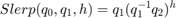
The original formulation of quaternion SLERP was given by Ken Shoemake [ 1] as:
An alternate formulation with sinusoids (used in the slerp function implementation) is:
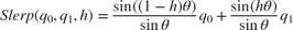
where  is the dot product of the quaternion parts. Note that
  .
.
SLERP vs Linear Interpolation of Quaternion Parts
Consider the following example. Build two quaternions from Euler angles.
q0 = quaternion([-80 10 0], 'eulerd', 'ZYX', 'frame');
q1 = quaternion([80 70 70], 'eulerd', 'ZYX', 'frame');
To find a quaternion 30 percent of the way from q0 to q1, specify the slerp parameter as 0.3.
p30 = slerp(q0, q1, 0.3);
To view the interpolated quaternion's Euler angle representation, use the eulerd function.
eulerd(p30, 'ZYX', 'frame')
ans =

  -56.6792   33.2464   -9.6740
To create a smooth trajectory between q0 and q1, specify the slerp interpolation parameter as a vector of evenly spaced numbers between 0 and 1.
dt = 0.01;
h = (0:dt:1).';
trajSlerped = slerp(q0, q1, h);
Compare the results of the SLERP algorithm with a trajectory between q0 and q1, using simple linear interpolation (LERP) of each quaternion part.
partsLinInterp = interp1( [0;1], compact([q0;q1]), h, 'linear');
Note that linear interpolation does not give unit quaternions, so they must be normalized.
trajLerped = normalize(quaternion(partsLinInterp));
Compute the angular velocities from each approach.
avSlerp = helperQuat2AV(trajSlerped, dt);
avLerp = helperQuat2AV(trajLerped, dt);
Plot both sets of angular velocities. Notice that the angular velocity for SLERP is constant, but it varies for linear interpolation.
sp = HelperSlerpPlotting;
sp.plotAngularVelocities(avSlerp, avLerp);
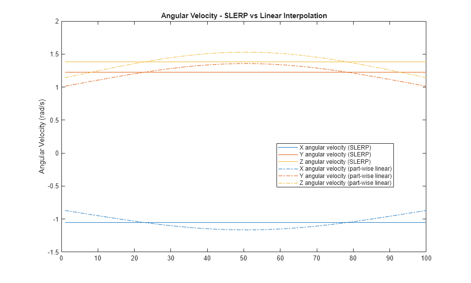
SLERP produces a smooth rotation at a constant rate.
Lowpass Filtering with SLERP
SLERP can also be used to make more complex functions. Here, SLERP is used to lowpass filter a noisy trajectory.
Rotational noise can be constructed by forming a quaternion from a noisy rotation vector.
rcurr = rng(1);
sigma = 1e-1;
noiserv = sigma .* ( rand(numel(h), 3) - 0.5);
qnoise = quaternion(noiserv, 'rotvec');
rng(rcurr);
To corrupt the trajectory trajSlerped with noise, incrementally rotate the trajectory with the noise vector qnoise.
trajNoisy = trajSlerped .* qnoise;
You can smooth real-valued signals using a single pole filter of the form:

This formula essentially says that the new filter state  should be moved toward the current input
  by a step size that is proportional to the distance between the current input and the current filter state
  .
.
The spirit of this approach informs how a quaternion sequence can be lowpass filtered. To do this, both the dist and slerp functions are used.
The dist function returns a measurement in radians of the difference in rotation applied by two quaternions. The range of the dist function is the half-open interval [0, pi).
The slerp function is used to steer the filter state towards the current input. It is steered more towards the input when the difference between the input and current filter state has a large dist, and less toward the input when dist gives a small value. The interpolation parameter to slerp is in the closed-interval [0,1], so the output of dist must be re-normalized to this range. However, the full range of [0,1] for the interpolation parameter gives poor performance, so it is limited to a smaller range hrange centered at hbias.
hrange = 0.4;
hbias = 0.4;
Limit low and high to the interval [0, 1].
low  = max(min(hbias - (hrange./2), 1), 0);
high = max(min(hbias + (hrange./2), 1), 0);
hrangeLimited = high - low;
Initialize the filter and preallocate outputs.
y = trajNoisy(1); % initial filter state
qout = zeros(size(y), 'like', y); % preallocate filter output
qout(1) = y;
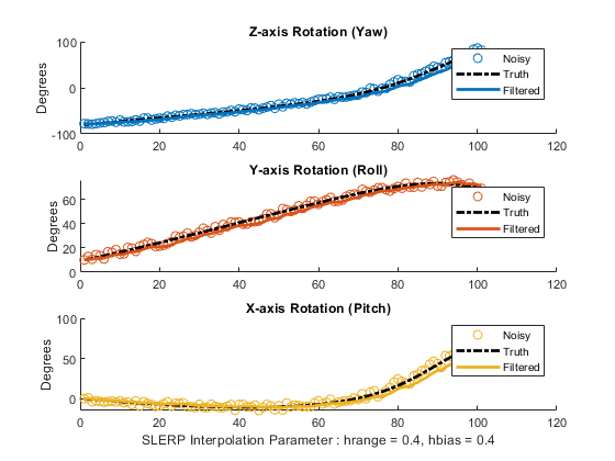
Filter the noisy trajectory, sample-by-sample.
for ii=2:numel(trajNoisy)
    x = trajNoisy(ii);
    d = dist(y, x);

    % Renormalize dist output to the range [low, high]
    hlpf = (d./pi).*hrangeLimited + low;
    y = slerp(y,x,hlpf);
    qout(ii) = y;
end

f = figure;
sp.plotEulerd(f, trajNoisy, 'o');
sp.plotEulerd(f, trajSlerped, 'k-.', 'LineWidth', 2);
sp.plotEulerd(f, qout, '-', 'LineWidth', 2);
sp.addAnnotations(f, hrange, hbias);

Conclusion
SLERP can be used for creating both short trajectories between two orientations and for smoothing or lowpass filtering. It has found widespread use in a variety of industries.
References
Shoemake, Ken. "Animating Rotation with Quaternion Curves." ACM SIGRAPH Computer Graphics 19, no 3 (1985):245-54, doi:10.1145/325165.325242