Multiplatform Radar Detection Generation
This example shows how to generate radar detections from a multiplatform radar network. The network includes three long-range platforms: two airborne and one ground-based. Such synthetic data can be used to test the performance of tracking architectures for different target types and maneuvers.
The radar platforms and targets are modeled in the scenario as platforms. Simulation of the motion of the platforms in the scenario is managed by trackingScenario.
% Create a tracking scenario to manage the movement of the platforms.
scene = trackingScenario;                % Create tracking scenario
scene.UpdateRate = 0;                    % Use continuous update rate to handle sensors with different update rates
sceneDuration = 60;                      % Duration of scenario in seconds
scene.StopTime = sceneDuration;
Airborne Platform with Rotating Radar Array
Add an airborne platform to the scenario traveling north at 650 km/hr at a cruising altitude of 10 km. Generate the platform trajectory from waypoints using waypointTrajectory.
ht = 10e3;                               % Altitude in meters
spd = 650*1e3/3600;                      % Speed in m/s
start = [-spd*sceneDuration/2 5e3 -ht];
stop  =  [spd*sceneDuration/2 5e3 -ht];
traj  = waypointTrajectory('Waypoints',[start;stop],'TimeOfArrival',[0; sceneDuration]);

% Create the airborne platform with its trajectory.
plat1 = platform(scene,'Trajectory',traj);
Add a planar array radar to the platform. Mount the radar in a radome 5 meters above the platform. Model the radar as a mechanically rotating phased array. The radar electronically stacks beams in elevation along the array's boresight. The specifications for the modeled radar are tabulated below:
Sensitivity: 0 dBsm @ 375 km
Mechanical Scan: Azimuth only
Mechanical Scan Limits: 0 to 360 deg
Electronic Scan: Elevation only
Electronic Scan Limits: -2 to 45 deg
Field of View: 1 deg azimuth, 47 deg elevation
Measurements: Azimuth, elevation, range
Azimuth Resolution: 1 deg
Elevation Resolution: 5 deg
Range Resolution: 30 m
Model the mechanically rotating radar using fusionRadarSensor.
sensorIndex = 1; % Identifies originating sensor of each detection
radar = fusionRadarSensor(sensorIndex,'Rotator', ...
    'MountingLocation', [0 0 -5], ...    % m
    'UpdateRate', 12.5, ...              % Hz
    'ReferenceRCS', 0, ...               % dBsm
    'ReferenceRange', 375e3, ...         % m
    'ScanMode', 'Mechanical and electronic', ...
    'MechanicalAzimuthLimits', [0 360], ...   % deg
    'MechanicalElevationLimits', [0 0], ...   % deg
    'ElectronicAzimuthLimits', [0 0], ...
    'ElectronicElevationLimits', [-2 45], ... % deg
    'FieldOfView',[1;47.1], ...               % deg
    'HasElevation', true, ...
    'AzimuthResolution', 1, ...               % deg
    'ElevationResolution', 5, ...             % deg
    'RangeResolution', 30, ...                % m
    'HasINS', true);

% Attach the radar to its airborne platform.
plat1.Sensors = radar;
Note, to model a radar system that does not perform scanning in one of the angular dimensions the field of view in that dimension should be set to a value that is slightly larger than the value spanned by the corresponding mechanical scan limits. Thus, in this example the elevation field of view of the fusionRadarSensor object is set to 47.1 degrees, while according to the specification the elevation field of view of the modeled system is 47 degrees.
Airborne Platform with Two Radar Arrays
Add a second airborne platform to the scenario traveling south at 550 km/hr at a cruising altitude of 8 km.
ht = 8e3;                                % Altitude in meters
spd = 550*1e3/3600;                      % Speed in m/s
start =  [spd*sceneDuration/2 5e3 -ht];
stop  = [-spd*sceneDuration/2 5e3 -ht];
traj  = waypointTrajectory('Waypoints',[start;stop],'TimeOfArrival',[0; sceneDuration]);
plat2 = platform(scene,'Trajectory',traj);
Multiple sensors can be mounted on a platform. Add a radar composed of two linear phased arrays mounted 5 meters above the platform. Mount the arrays so that one array looks over the right side of the airframe and the other array looks over the left side of the airframe. Both arrays provide coverage over a 150 degree azimuth sector on either side of the platform. Elevation is not measured by the linear arrays. The specifications for this radar are tabulated below:
Sensitivity: 0 dBsm @ 350 km
Mechanical Scan: No
Electronic Scan: Azimuth only
Electronic Scan Limits: -75 to 75 deg
Field of View: 1 deg azimuth, 60 deg elevation
Measurements: Azimuth, range
Azimuth Resolution: 1 deg
Range Resolution: 30 m
Model the linear phased array radar using the fusionRadarSensor.
% Create right facing radar by setting radar's yaw to 90 degrees.
sensorIndex = sensorIndex+1;
rightRadar = fusionRadarSensor(sensorIndex,'Sector', ...
    'MountingLocation', [0 0 -5], ...    % m
    'MountingAngles', [90 0 0], ...      % deg, look over right side
    'UpdateRate', 12.5, ...              % Hz
    'ReferenceRCS', 0, ...               % dBsm
    'ReferenceRange', 350e3, ...         % m
    'ScanMode','Electronic', ...
    'ElectronicAzimuthLimits',[-75 75], ... % deg
    'FieldOfView',[1;60], ...               % deg
    'HasElevation', false, ...
    'AzimuthResolution', 1, ...             % deg
    'RangeResolution', 30, ...              % m
    'HasINS', true);

% Create an identical radar looking over the left side of the airframe.
leftRadar = clone(rightRadar);
sensorIndex = sensorIndex+1;
leftRadar.SensorIndex = sensorIndex;
leftRadar.MountingAngles(1) = -90; % Look over the left side

% Attach the two linear radar arrays to the airborne platform.
plat2.Sensors = {leftRadar, rightRadar};
Ground-Based Platform with Rectangular Radar Array
Add a ground-based radar using a rectangular phased array mounted 5 meters above its trailer. The radar electronically surveys a 60 degree azimuth span and 20 degrees of elevation above the ground using an electronic raster scan pattern.
Sensitivity: 0 dBsm @ 350 km
Mechanical Scan: No
Electronic Scan: Azimuth and elevation
Electronic Scan Limits: -30 to 30 deg azimuth, -20 to 0 deg elevation
Field of View: 1 deg azimuth, 5 deg elevation
Measurements: Azimuth, elevation, range
Azimuth Resolution: 1 deg
Elevation Resolution: 5 deg
Range Resolution: 30 m
Model the rectangular phased array radar using the fusionRadarSensor.
% Create an electronically scanning rectangular array radar.
sensorIndex = sensorIndex+1;
radar = fusionRadarSensor(sensorIndex,'Raster', ...
    'MountingLocation', [0 0 -5], ...    % m
    'UpdateRate', 25, ...                % Hz
    'ReferenceRCS', 0, ...               % dBsm
    'ReferenceRange', 350e3, ...         % m
    'ScanMode','Electronic', ...
    'ElectronicAzimuthLimits', [-30 30],... % deg
    'ElectronicElevationLimits', [-20 0],... % deg
    'FieldOfView', [1;5], ...            % deg
    'HasElevation', true, ...
    'AzimuthResolution', 1, ...          % deg
    'ElevationResolution', 5, ...        % deg
    'RangeResolution', 30, ...           % m
    'HasINS', true);

% Attach the rectangular radar array to the trailer platform.
plat3 = platform(scene,'Sensors',radar);
plat3.Trajectory.Position = [-30e3 30e3 0];
plat3.Trajectory.Orientation = quaternion([-60 0 0],'eulerd','zyx','frame');
Airborne Targets
Add four airborne targets within the surveillance region.
Airliner traveling northeast at 700 km/hr at a 3,000 m altitude
Crossing airliner traveling southeast at 900 km/hr at a 4,000 m altitude
Airliner traveling east at 600 km/hr at a 9,000 m altitude
Jet traveling at 300 km/hr and executing a 90 degree turn at a 3,000 m altitude
% Add airliner traveling northeast.
ht = 3e3;                                % Altitude in meters
spd = 700*1e3/3600;                      % Speed in m/s
ang = 45;
rot = [cosd(ang) sind(ang) 0;-sind(ang) cosd(ang) 0; 0 0 1];
offset = [-15e3 -25e3 -ht];
start = offset - [spd*sceneDuration/2 0 0]*rot;
stop  = offset + [spd*sceneDuration/2 0 0]*rot;
traj  = waypointTrajectory('Waypoints',[start;stop],'TimeOfArrival',[0; sceneDuration]);

rcs = rcsSignature('Pattern', [10 10; 10 10], ...
        'Azimuth', [-180 180], 'Elevation', [-90 90], ...
        'Frequency', [0 10e9]);          % Define custom RCS signature of target
platform(scene,'Trajectory',traj,'Signatures',rcs);

% Add crossing airliner traveling southeast.
ht = 4e3;                                % Altitude in meters
spd = 900*1e3/3600;                      % Speed in m/s
offset = [(start(1)+stop(1))/2 (start(2)+stop(2))/2 -ht];
start = offset + [0 -spd*sceneDuration/2 0]*rot;
stop  = offset + [0  spd*sceneDuration/2 0]*rot;
traj  = waypointTrajectory('Waypoints',[start;stop],'TimeOfArrival',[0; sceneDuration]);
rcs = rcsSignature;                      % Default 10 dBsm RCS at all viewing angles
platform(scene,'Trajectory',traj,'Signatures',rcs);

% Add eastbound airliner.
ht = 9e3;                                % Altitude in meters
spd = 600*1e3/3600;                      % Speed in m/s
start = [30e3 -spd*sceneDuration/2-20e3 -ht];
stop  = [30e3  spd*sceneDuration/2-20e3 -ht];
traj  = waypointTrajectory('Waypoints',[start;stop],'TimeOfArrival',[0; sceneDuration]);
platform(scene,'Trajectory',traj);       % Default 10 dBsm RCS at all viewing angles

% Add jet turning with horizontal acceleration of 0.3 G.
ht = 3e3;                                % Altitude in meters
spd = 300*1e3/3600;                      % Speed in m/s
accel = 0.3*9.8;                         % Centripetal acceleration m/s^2
radius = spd^2/accel;                    % Turn radius in meters
t0 = 0;
t1 = t0+5;
t2 = t1+pi/2*radius/spd;
t3 = sceneDuration;
start = [0e4 -4e4 -ht];
wps = [ ...
    0                   0                   0; ... % Begin straight segment
    spd*t1              0                   0; ... % Begin horizontal turn
    spd*t1+radius       radius              0; ... % End of horizontal turn
    spd*t1+radius       radius+spd*(t3-t2)  0];    % End of second straight segment
traj  = waypointTrajectory('Waypoints',start+wps,'TimeOfArrival',[t0; t1; t2; t3]);
platform(scene,'Trajectory',traj);
Generation of Radar Detections
The following loop advances the platform and target positions until the end of the scenario. For each step forward in the scenario, detections are generated from each platform.
The trackingScenario can advance at a fixed time interval or automatically determine the next update time. Set the UpdateRate to 0 to let trackingScenario determine the next update time.
rng(2018); % Set random seed for repeatable results

% Create a theaterPlot to show the true and measured positions of the detected targets and platforms.
theaterDisplay = helperMultiPlatDisplay(scene);

title('Multiplatform Radar Scenario');
legend('show');

% Show 3D view of the scenario.
view(-60,10);

% Log all the detections
detLog = {};
timeLog = [];

while advance(scene)
    % Generate detections from radars on each platform.
    [dets,configs] = detect(scene);

    % Update display with current beam positions and detections.
    theaterDisplay(dets);

    % Log sensor data and ground truth.
    detLog = [detLog; dets]; %#ok<AGROW>
    timeLog = [timeLog; scene.SimulationTime];%#ok<AGROW>
end
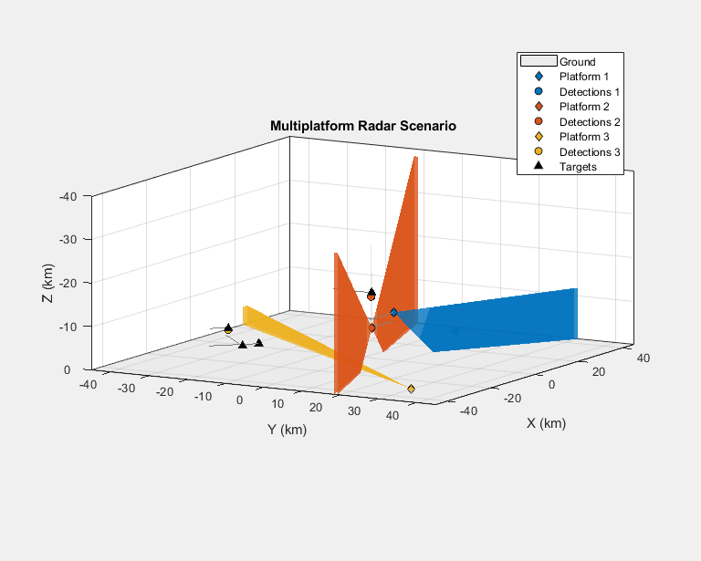
Notice the wide beams from the airborne platforms and the narrow beam from the ground-based radar executing a raster scan. You can visualize the ground truth trajectories in the 2D view below. The four targets are represented by triangles. Around 30 km on the x-axis is the airliner traveling east (left to right). Around 2 km on the x-axis is the jet executing a turn clockwise. Further south are two crossing airliners.
view(-90,90); % 2D view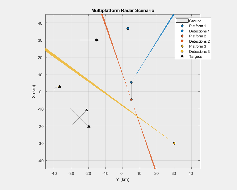
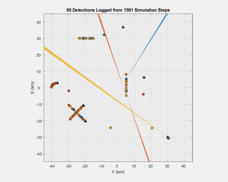
Plot the logged detections with their measurement uncertainties. Each color corresponds to the platform generating the detections. The legend from the previous display applies to all the following plots. Notice that the radars generate false alarms, which are detection far away from the target trajectories.
theaterDisplay(detLog);
title([num2str(numel(detLog)) ' Detections Logged from ' num2str(numel(timeLog)) ' Simulation Steps']);
legend('hide');
The following 3D view shows how these detections are distributed in elevation. For platforms with 3D sensors (the blue and yellow platforms), the detections closely follow the target trajectories. The 2D-view platform's detections (the red platform) are offset in elevation from the target trajectories because its radar is unable to measure in elevation. The 1-sigma measurement uncertainty is shown for each detection as a gray ellipsoid centered on the measured target positions (shown as filled circles).
view([-60 25]); % 3D view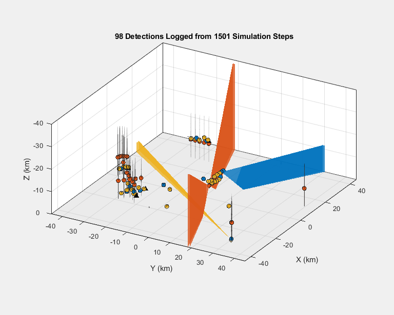
Zoom in on the jet executing the 90 degree horizontal turn. The 1-sigma measurement uncertainty is reported by the radar according to the radar's resolution and the signal-to-noise ratio (SNR) for each detection. Targets at longer ranges or with smaller SNR values will have larger measurement uncertainties than targets at closer ranges or with larger SNR values. Notice that the blue detections have smaller measurement uncertainties than the yellow detections. This is because the blue detections originate from the airborne platform (Platform 1) that is much closer to the target than the ground-based platform (Platform 3) generating the yellow detections.
xlim([-3000 9000]); ylim([-44000 -32000]); zlim([-12000 0000]);
axis('square');
title('Jet Executing Horizontal Turn');
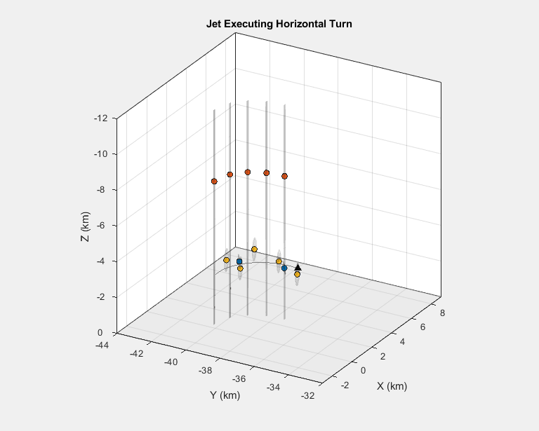
Notice the large uncertainty in elevation of the red detections generating from the airborne platform (Platform 2) that uses two linear arrays. The ellipsoids have small axes in the range and azimuth directions but have very large axes along the elevation direction. This is because the linear arrays on this platform are unable to provide estimates in elevation. In this case, the platform's radar reports detections at 0 degrees with an uncertainty in elevation corresponding to the elevation field of view.
Zoom in on the two crossing airliners. The blue airborne radar with the rotating array generates the fewest number of detections (only 4 detections for these two targets), but these detections are the most precise (smallest ellipses). The small number of detections from this platform is due to its radar's 360 mechanical scan, which limits how frequently its beam can revisit a target in the scenario. The other platforms have radars with smaller scan regions, allowing them to revisit the targets at a higher rate.
view([-55 20]);
xlim([-22000 -10000]); ylim([-31000 -19000]);
title('Crossing Airliners');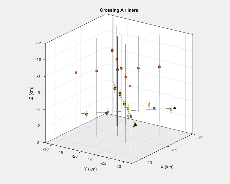
Zoom in on the airliner traveling east. Same observations on the number of detections and accuracy from different radar platforms apply.
view([-70 10]);
xlim([24000 36000]); ylim([-26000 -14000]); zlim([-15000 -3000])
title('Airliner Traveling East');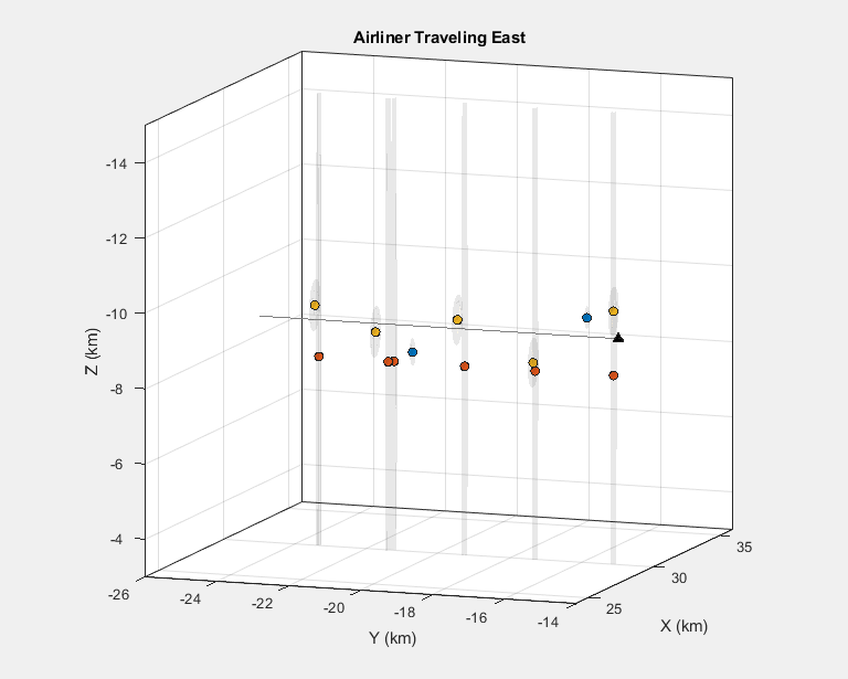
Summary
This example shows how to model a radar surveillance network and simulate detections generated by multiple airborne and ground-based radar platforms. In this example, you learned how to define scenarios, including targets and platforms that can be stationary or in motion. You also learned how to visualize the ground truth trajectories, sensor beams, detections, and associated measurement uncertainties. You can process this synthetic data through your tracking and fusion algorithms to assess their performance for this scenario. You can also modify this example to exercise your multi-target tracker against different target types and maneuvers.