Track Vehicles Using Lidar: From Point Cloud to Track List

This example uses:

This example shows how to track vehicles using measurements from a lidar sensor mounted on top of an ego vehicle. Lidar sensors report measurements as a point cloud. The example illustrates the workflow in MATLAB® for processing the point cloud and tracking the objects. For a Simulink® version of the example, refer to Track Vehicles Using Lidar Data in Simulink.The lidar data used in this example is recorded from a highway driving scenario. In this example, you use the recorded data to track vehicles with a joint probabilistic data association (JPDA) tracker and an interacting multiple model (IMM) approach.

3-D Bounding Box Detector Model

Due to high resolution capabilities of the lidar sensor, each scan from the sensor contains a large number of points, commonly known as a point cloud. This raw data must be preprocessed to extract objects of interest, such as cars, cyclists, and pedestrians. In this example, you use a classical segmentation algorithm using a distance-based clustering algorithm. For more details about segmentation of lidar data into objects such as the ground plane and obstacles, refer to the Ground Plane and Obstacle Detection Using Lidar (Automated Driving Toolbox) example. For a deep learning segmentation workflow, refer to the Detect, Classify, and Track Vehicles Using Lidar (Lidar Toolbox) example. In this example, the point clouds belonging to obstacles are further classified into clusters using the pcsegdist function, and each cluster is converted to a bounding box detection with the following format:

$[x\ y\ z\ {\theta}\ l\ w\ h]$

$x$ , $y$ and $z$ refer to the x-, y- and z-positions of the bounding box, ${\theta}$ refers to its yaw angle and $l$ , $w$ and $h$ refer to its length, width, and height, respectively. The pcfitcuboid (Lidar Toolbox) function uses L-shape fitting algorithm to determine the yaw angle of the bounding box.

The detector is implemented by a supporting class HelperBoundingBoxDetector, which wraps around point cloud segmentation and clustering functionalities. An object of this class accepts a pointCloud input and returns a list of objectDetection objects with bounding box measurements.

The diagram shows the processes involved in the bounding box detector model and the Lidar Toolbox™ functions used to implement each process. It also shows the properties of the supporting class that control each process.

The lidar data is available at the following location: https://ssd.mathworks.com/supportfiles/lidar/data/TrackVehiclesUsingLidarExampleData.zip

Download the data files into your temporary directory, whose location is specified by MATLAB's tempdir function. If you want to place the files in a different folder, change the directory name in the subsequent instructions.

% Load data if unavailable. The lidar data is stored as a cell array of
% pointCloud objects.
if ~exist('lidarData','var')
    dataURL = 'https://ssd.mathworks.com/supportfiles/lidar/data/TrackVehiclesUsingLidarExampleData.zip';
    datasetFolder = fullfile(tempdir,'LidarExampleDataset');
    if ~exist(datasetFolder,'dir') || numel(dir(fullfile(datasetFolder,"*.mat"))) ~= 6
       unzip(dataURL,datasetFolder);
    end
    % Specify initial and final time for simulation.
    initTime = 0;
    finalTime = 35;
    [lidarData, imageData] = loadLidarAndImageData(datasetFolder,initTime,finalTime);
end

% Set random seed to generate reproducible results.
S = rng(2018);

% A bounding box detector model.
detectorModel = HelperBoundingBoxDetector(...
    'XLimits',[-50 75],...              % min-max
    'YLimits',[-5 5],...                % min-max
    'ZLimits',[-2 5],...                % min-max
    'SegmentationMinDistance',1.8,...   % minimum Euclidian distance
    'MinDetectionsPerCluster',1,...     % minimum points per cluster
    'MeasurementNoise',blkdiag(0.25*eye(3),25,eye(3)),...       % measurement noise in detection report
    'GroundMaxDistance',0.3);           % maximum distance of ground points from ground plane

Target State and Sensor Measurement Model

The first step in tracking an object is defining its state, and the models that define the transition of state and the corresponding measurement. These two sets of equations are collectively known as the state-space model of the target. To model the state of vehicles for tracking using lidar, this example uses a cuboid model with following convention:

$x = [x_{kin}\ {\theta}\ l\ w\ h]$

$x_{kin}$ refers to the portion of the state that controls the kinematics of the motion center, and $\theta$ is the yaw angle. The length, width, and height of the cuboid are modeled as constants, whose estimates evolve in time during correction stages of the filter.

In this example, you use two state-space models: a constant velocity (cv) cuboid model and a constant turn-rate (ct) cuboid model. These models differ in the way they define the kinematic part of the state, as described below:

$x_{cv} = [x\ {\dot{x}}\ y\ {\dot{y}}\ z\ {\dot{z}}\ {\theta}\ l\ w\ h]$

$x_{ct} = [x\ {\dot{x}}\ y\ {\dot{y}}\ {\dot{\theta}}\ z\ {\dot{z}}\ {\theta}\ l\ w\ h]$

For information about their state transition, refer to the helperConstvelCuboid and helperConstturnCuboid functions used in this example.

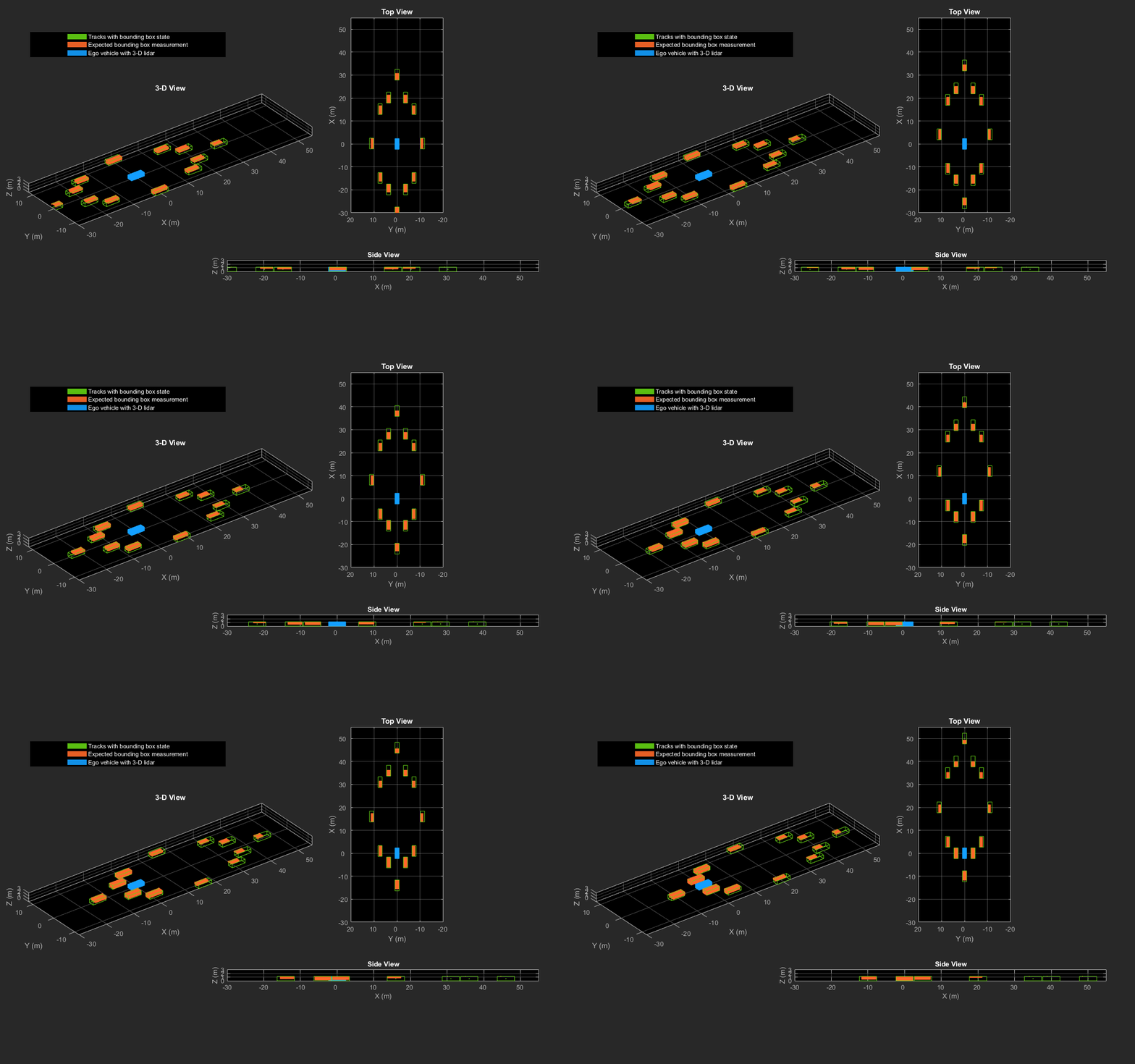
The helperCvmeasCuboid and helperCtmeasCuboid measurement models describe how the sensor perceives the constant velocity and constant turn-rate states respectively, and they return bounding box measurements. Because the state contains information about size of the target, the measurement model includes the effect of center-point offset and bounding box shrinkage, as perceived by the sensor, due to effects like self-occlusion [1]. This effect is modeled by a shrinkage factor that is directly proportional to the distance from the tracked vehicle to the sensor.

The image below demonstrates the measurement model operating at different state-space samples. Notice the modeled effects of bounding box shrinkage and center-point offset as the objects move around the ego vehicle.

Set Up Tracker and Visualization

The image below shows the complete workflow to obtain a list of tracks from a pointCloud input.

Now, set up the tracker and the visualization used in the example.

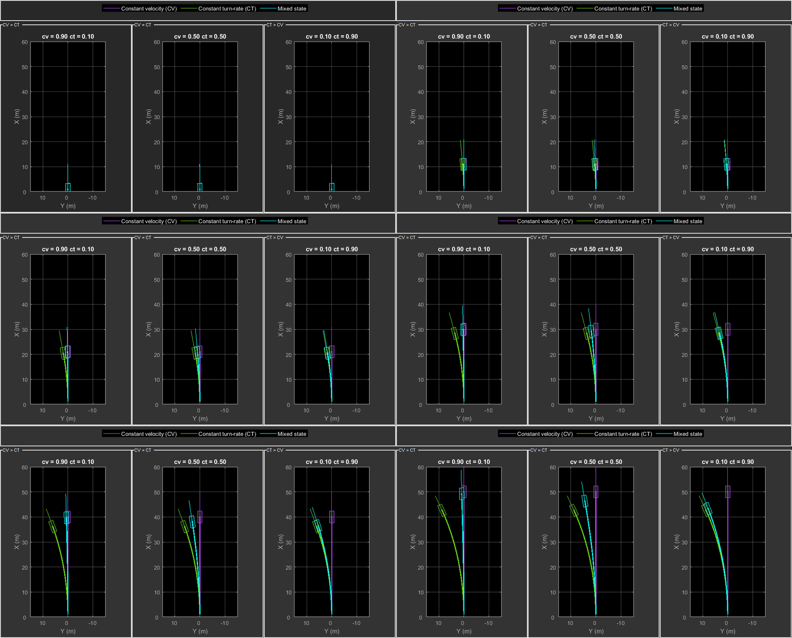
A joint probabilistic data association tracker (trackerJPDA) coupled with an IMM filter (trackingIMM) is used to track objects in this example. The IMM filter uses a constant velocity and constant turn-rate model and is initialized using the supporting function, helperInitIMMFilter, included with this example. The IMM approach helps a track to switch between motion models and thus achieve good estimation accuracy during events like maneuvering or lane changing. The animation below shows the effect of mixing the constant velocity and constant turn-rate model during prediction stages of the IMM filter.

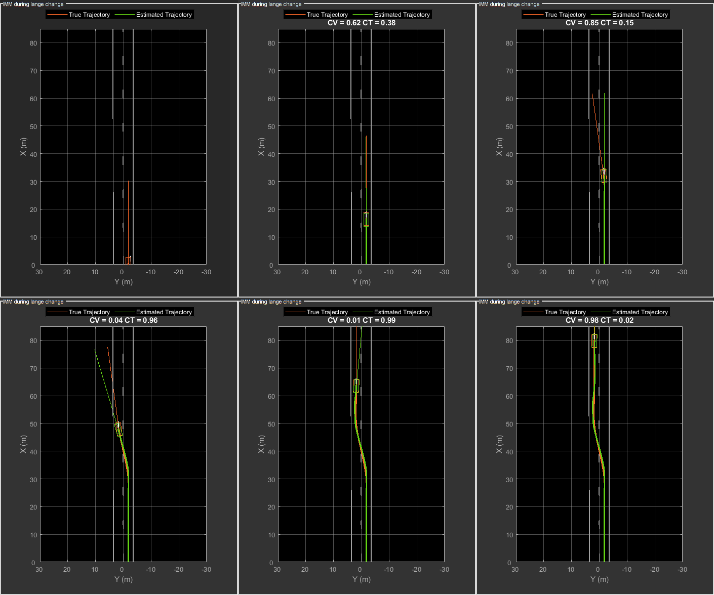
The IMM filter updates the probability of each model when it is corrected with detections from the object. The animation below shows the estimated trajectory of a vehicle during a lane change event and the corresponding estimated probabilities of each model.

Set the HasDetectableTrackIDsInput property of the tracker as true, which enables you to specify a state-dependent probability of detection. The detection probability of a track is calculated by the helperCalcDetectability function, listed at the end of this example.

assignmentGate = [75 1000]; % Assignment threshold;
confThreshold = [7 10];    % Confirmation threshold for history logic
delThreshold = [8 10];     % Deletion threshold for history logic
Kc = 1e-9;                 % False-alarm rate per unit volume

% IMM filter initialization function
filterInitFcn = @helperInitIMMFilter;

% A joint probabilistic data association tracker with IMM filter
tracker = trackerJPDA('FilterInitializationFcn',filterInitFcn,...
    'TrackLogic','History',...
    'AssignmentThreshold',assignmentGate,...
    'ClutterDensity',Kc,...
    'ConfirmationThreshold',confThreshold,...
    'DeletionThreshold',delThreshold,...
    'HasDetectableTrackIDsInput',true,...
    'InitializationThreshold',0,...
    'HitMissThreshold',0.1);

The visualization is divided into these main categories:

Lidar Preprocessing and Tracking - This display shows the raw point cloud, segmented ground, and obstacles. It also shows the resulting detections from the detector model and the tracks of vehicles generated by the tracker.
Ego Vehicle Display - This display shows the 2-D bird's-eye view of the scenario. It shows the obstacle point cloud, bounding box detections, and the tracks generated by the tracker. For reference, it also displays the image recorded from a camera mounted on the ego vehicle and its field of view.
Tracking Details - This display shows the scenario zoomed around the ego vehicle. It also shows finer tracking details, such as error covariance in estimated position of each track and its motion model probabilities, denoted by cv and ct.

% Create display
displayObject = HelperLidarExampleDisplay(imageData{1},...
    'PositionIndex',[1 3 6],...
    'VelocityIndex',[2 4 7],...
    'DimensionIndex',[9 10 11],...
    'YawIndex',8,...
    'MovieName','',...  % Specify a movie name to record a movie.
    'RecordGIF',false); % Specify true to record new GIFs

Loop Through Data

Loop through the recorded lidar data, generate detections from the current point cloud using the detector model and then process the detections using the tracker.

time = 0;       % Start time
dT = 0.1;       % Time step

% Initiate all tracks.
allTracks = struct([]);

% Initiate variables for comparing MATLAB and MEX simulation.
numTracks = zeros(numel(lidarData),2);

% Loop through the data
for i = 1:numel(lidarData)
    % Update time
    time = time + dT;

    % Get current lidar scan
    currentLidar = lidarData{i};

    % Generator detections from lidar scan.
    [detections,obstacleIndices,groundIndices,croppedIndices] = detectorModel(currentLidar,time);

    % Calculate detectability of each track.
    detectableTracksInput = helperCalcDetectability(allTracks,[1 3 6]);

    % Pass detections to track.
    [confirmedTracks,tentativeTracks,allTracks,info] = tracker(detections,time,detectableTracksInput);
    numTracks(i,1) = numel(confirmedTracks);

    % Get model probabilities from IMM filter of each track using
    % getTrackFilterProperties function of the tracker.
    modelProbs = zeros(2,numel(confirmedTracks));
    for k = 1:numel(confirmedTracks)
        c1 = getTrackFilterProperties(tracker,confirmedTracks(k).TrackID,'ModelProbabilities');
        modelProbs(:,k) = c1{1};
    end

    % Update display
    if isvalid(displayObject.PointCloudProcessingDisplay.ObstaclePlotter)
        % Get current image scan for reference image
        currentImage = imageData{i};

        % Update display object
        displayObject(detections,confirmedTracks,currentLidar,obstacleIndices,...
            groundIndices,croppedIndices,currentImage,modelProbs);
    end

    % Snap a figure at time = 18
    if abs(time - 18) < dT/2
        snapnow(displayObject);
    end
end

% Write movie if requested
if ~isempty(displayObject.MovieName)
    writeMovie(displayObject);
end

% Write new GIFs if requested.
if displayObject.RecordGIF
    % second input is start frame, third input is end frame and last input
    % is a character vector specifying the panel to record.
    writeAnimatedGIF(displayObject,10,170,'trackMaintenance','ego');
    writeAnimatedGIF(displayObject,310,330,'jpda','processing');
    writeAnimatedGIF(displayObject,120,140,'imm','details');
end

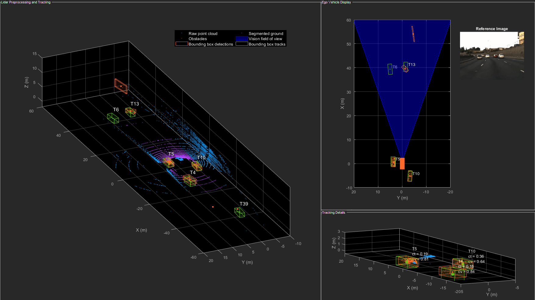
The figure above shows the three displays at time = 18 seconds. The tracks are represented by green bounding boxes. The bounding box detections are represented by orange bounding boxes. The detections also have orange points inside them, representing the point cloud segmented as obstacles. The segmented ground is shown in purple. The cropped or discarded point cloud is shown in blue.

Generate C Code

You can generate C code from the MATLAB® code for the tracking and the preprocessing algorithm using MATLAB Coder™. C code generation enables you to accelerate MATLAB code for simulation. To generate C code, the algorithm must be restructured as a MATLAB function, which can be compiled into a MEX file or a shared library. For this purpose, the point cloud processing algorithm and the tracking algorithm is restructured into a MATLAB function, mexLidarTracker. Some variables are defined as persistent to preserve their state between multiple calls to the function (see persistent). The inputs and outputs of the function can be observed in the function description provided in the "Supporting Files" section at the end of this example.

MATLAB Coder requires specifying the properties of all the input arguments. An easy way to do this is by defining the input properties by example at the command line using the -args option. For more information, see Specify Input Types at the Command Line (MATLAB Coder). Note that the top-level input arguments cannot be objects of the handle class. Therefore, the function accepts the x, y and z locations of the point cloud as an input. From the stored point cloud, this information can be extracted using the Location property of the pointCloud object. This information is also directly available as the raw data from the lidar sensor.

% Input lists
inputExample = {lidarData{1}.Location, 0};

% Create configuration for MEX generation
cfg = coder.config('mex');

% Replace cfg with the following to generate static library and perform
% software-in-the-loop simulation. This requires an Embedded Coder license.
%
% cfg = coder.config('lib'); % Static library
% cfg.VerificationMode = 'SIL'; % Software-in-the-loop

% Generate code if file does not exist.
if ~exist('mexLidarTracker_mex','file')
    h = msgbox({'Generating code. This may take a few minutes...';'This message box will close when done.'},'Codegen Message');
    % -config allows specifying the codegen configuration
    % -o allows specifying the name of the output file
    codegen -config cfg -o mexLidarTracker_mex mexLidarTracker -args inputExample
    close(h);
else
    clear mexLidarTracker_mex;
end

Code generation successful.

Rerun simulation with MEX Code

Rerun the simulation using the generated MEX code, mexLidarTracker_mex. Reset time

time = 0;

for i = 1:numel(lidarData)
    time = time + dT;

    currentLidar = lidarData{i};

    [detectionsMex,obstacleIndicesMex,groundIndicesMex,croppedIndicesMex,...
        confirmedTracksMex, modelProbsMex] = mexLidarTracker_mex(currentLidar.Location,time);

    % Record data for comparison with MATLAB execution.
    numTracks(i,2) = numel(confirmedTracksMex);
end

Compare results between MATLAB and MEX Execution

disp(isequal(numTracks(:,1),numTracks(:,2)));

Notice that the number of confirmed tracks is the same for MATLAB and MEX code execution. This assures that the lidar preprocessing and tracking algorithm returns the same results with generated C code as with the MATLAB code.

Results

Now, analyze different events in the scenario and understand how the combination of lidar measurement model, joint probabilistic data association, and interacting multiple model filter, helps achieve a good estimation of the vehicle tracks.

Track Maintenance

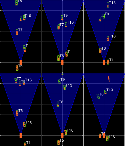
The animation above shows the simulation between time = 3 seconds and time = 16 seconds. Notice that tracks such as T10 and T6 maintain their IDs and trajectory during the time span. However, track T9 is lost because the tracked vehicle was missed (not detected) for a long time by the sensor. Also, notice that the tracked objects are able to maintain their shape and kinematic center by positioning the detections onto the visible portions of the vehicles. For example, as Track T7 moves forward, bounding box detections start to fall on its visible rear portion and the track maintains the actual size of the vehicle. This illustrates the offset and shrinkage effect modeled in the measurement functions.

Capturing Maneuvers

The animation shows that using an IMM filter helps the tracker to maintain tracks on maneuvering vehicles. Notice that the vehicle tracked by T4 changes lanes behind the ego vehicle. The tracker is able maintain a track on the vehicle during this maneuvering event. Also notice in the display that its probability of following the constant turn model, denoted by ct, increases during the lane change maneuver.

Joint Probabilistic Data Association

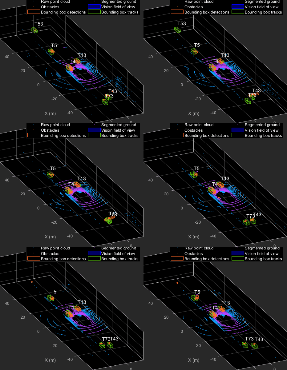
This animation shows that using a joint probabilistic data association tracker helps in maintaining tracks during ambiguous situations. Here, vehicles tracked by T43 and T73, have a low probability of detection due to their large distance from the sensor. Notice that the tracker is able to maintain tracks during events when one of the vehicles is not detected. During the event, the tracks first coalesce, which is a known phenomenon in JPDA, and then separate as soon as the vehicle was detected again.

Summary

This example showed how to use a JPDA tracker with an IMM filter to track objects using a lidar sensor. You learned how a raw point cloud can be preprocessed to generate detections for conventional trackers, which assume one detection per object per sensor scan. You also learned how to define a cuboid model to describe the kinematics, dimensions, and measurements of extended objects being tracked by the JPDA tracker. In addition, you generated C code from the algorithm and verified its execution results with the MATLAB simulation.

Supporting Files

This section highlights the code from some important supporting files used in this example. The complete list of supporting files can be found in the current working directory after opening the example in MATLAB.

% *helperLidarModel*
%
% This function defines the lidar model to simulate shrinkage of the
% bounding box measurement and center-point offset. This function is used
% in the |helperCvmeasCuboid| and |helperCtmeasCuboid| functions to obtain
% bounding box measurement from the state.
%
% <include>helperLidarModel.m</include>
%

helperInverseLidarModel

This function defines the inverse lidar model to initiate a tracking filter using a lidar bounding box measurement. This function is used in the helperInitIMMFilter function to obtain state estimates from a bounding box measurement.

function [pos,posCov,dim,dimCov,yaw,yawCov] = helperInverseLidarModel(meas,measCov)
% This function returns the position, dimension, yaw using a bounding
% box measurement.

% Copyright 2019 The MathWorks, Inc.

% Shrink rate.
s = 3/50;
sz = 2/50;

% x,y and z of measurement
x = meas(1,:);
y = meas(2,:);
z = meas(3,:);

[az,~,r] = cart2sph(x,y,z);

% Shift x and y position.
Lshrink = abs(s*r.*(cos(az)));
Wshrink = abs(s*r.*(sin(az)));
Hshrink = sz*r;

shiftX = Lshrink;
shiftY = Wshrink;
shiftZ = Hshrink;

x = x + sign(x).*shiftX/2;
y = y + sign(y).*shiftY/2;
z = z - shiftZ/2;

pos = [x;y;z];
posCov = measCov(1:3,1:3,:);

yaw = meas(4,:);
yawCov = measCov(4,4,:);

% Dimensions are initialized for a standard passenger car with low
% uncertainity.
dim = [4.7;1.8;1.4];
dimCov = 0.01*eye(3);
end

HelperBoundingBoxDetector

This is the supporting class HelperBoundingBoxDetector to accept a point cloud input and return a list of objectDetection

classdef HelperBoundingBoxDetector < matlab.System
    % HelperBoundingBoxDetector A helper class to segment the point cloud
    % into bounding box detections.
    % The step call to the object does the following things:
    %
    % 1. Removes point cloud outside the limits.
    % 2. From the survived point cloud, segments out ground
    % 3. From the obstacle point cloud, forms clusters and puts bounding
    %    box on each cluster.
    
    % Cropping properties
    properties
        % XLimits XLimits for the scene
        XLimits = [-70 70];
        % YLimits YLimits for the scene
        YLimits = [-6 6];
        % ZLimits ZLimits for the scene
        ZLimits = [-2 10];
    end
   
    % Ground Segmentation Properties
    properties
        % GroundMaxDistance Maximum distance of point to the ground plane
        GroundMaxDistance = 0.3;
        % GroundReferenceVector Reference vector of ground plane
        GroundReferenceVector = [0 0 1];
        % GroundMaxAngularDistance Maximum angular distance of point to reference vector
        GroundMaxAngularDistance = 5;
    end
    
    % Bounding box Segmentation properties
    properties
        % SegmentationMinDistance Distance threshold for segmentation
        SegmentationMinDistance = 1.6;
        % MinDetectionsPerCluster Minimum number of detections per cluster
        MinDetectionsPerCluster = 2;
        % MaxZDistanceCluster Maximum Z-coordinate of cluster
        MaxZDistanceCluster = 3;
        % MinZDistanceCluster Minimum Z-coordinate of cluster
        MinZDistanceCluster = -3;
    end
    
    % Ego vehicle radius to remove ego vehicle point cloud.
    properties
        % EgoVehicleRadius Radius of ego vehicle
        EgoVehicleRadius = 3;
    end
    
    properties
        % MeasurementNoise Measurement noise for the bounding box detection
        MeasurementNoise = blkdiag(eye(3),10,eye(3));
    end
    
    properties (Nontunable)
        MeasurementParameters = struct.empty(0,1);
    end
    
    methods 
        function obj = HelperBoundingBoxDetector(varargin)
            setProperties(obj,nargin,varargin{:})
        end
    end
    
    methods (Access = protected)
        function [bboxDets,obstacleIndices,groundIndices,croppedIndices] = stepImpl(obj,currentPointCloud,time)
            % Crop point cloud
            [pcSurvived,survivedIndices,croppedIndices] = cropPointCloud(currentPointCloud,obj.XLimits,obj.YLimits,obj.ZLimits,obj.EgoVehicleRadius);
            % Remove ground plane
            [pcObstacles,obstacleIndices,groundIndices] = removeGroundPlane(pcSurvived,obj.GroundMaxDistance,obj.GroundReferenceVector,obj.GroundMaxAngularDistance,survivedIndices);
            % Form clusters and get bounding boxes
            detBBoxes = getBoundingBoxes(pcObstacles,obj.SegmentationMinDistance,obj.MinDetectionsPerCluster,obj.MaxZDistanceCluster,obj.MinZDistanceCluster);
            % Assemble detections
            if isempty(obj.MeasurementParameters)
                measParams = {};
            else
                measParams = obj.MeasurementParameters;
            end
            bboxDets = assembleDetections(detBBoxes,obj.MeasurementNoise,measParams,time);
        end
    end
end
    
function detections = assembleDetections(bboxes,measNoise,measParams,time)
% This method assembles the detections in objectDetection format.
numBoxes = size(bboxes,2);
detections = cell(numBoxes,1);
for i = 1:numBoxes
    detections{i} = objectDetection(time,cast(bboxes(:,i),'double'),...
        'MeasurementNoise',double(measNoise),'ObjectAttributes',struct,...
        'MeasurementParameters',measParams);
end
end

function bboxes = getBoundingBoxes(ptCloud,minDistance,minDetsPerCluster,maxZDistance,minZDistance)
    % This method fits bounding boxes on each cluster with some basic
    % rules.
    % Cluster must have at least minDetsPerCluster points.
    % Its mean z must be between maxZDistance and minZDistance.
    % length, width and height are calculated using min and max from each
    % dimension.
    [labels,numClusters] = pcsegdist(ptCloud,minDistance);
    pointData = ptCloud.Location;
    bboxes = nan(7,numClusters,'like',pointData);
    isValidCluster = false(1,numClusters);
    for i = 1:numClusters
        thisPointData = pointData(labels == i,:);
        meanPoint = mean(thisPointData,1);
        if size(thisPointData,1) > minDetsPerCluster && ...
                meanPoint(3) < maxZDistance && meanPoint(3) > minZDistance
            cuboid = pcfitcuboid(pointCloud(thisPointData));
            yaw = cuboid.Orientation(3);
            L = cuboid.Dimensions(1);
            W = cuboid.Dimensions(2);
            H = cuboid.Dimensions(3);
            if abs(yaw) > 45
                possibles = yaw + [-90;90];
                [~,toChoose] = min(abs(possibles));
                yaw = possibles(toChoose);
                temp = L;
                L = W;
                W = temp;
            end
            bboxes(:,i) = [cuboid.Center yaw L W H]';
            isValidCluster(i) = L < 20 & W < 20;
        end
    end
    bboxes = bboxes(:,isValidCluster);
end

function [ptCloudOut,obstacleIndices,groundIndices] = removeGroundPlane(ptCloudIn,maxGroundDist,referenceVector,maxAngularDist,currentIndices)
    % This method removes the ground plane from point cloud using
    % pcfitplane.
    [~,groundIndices,outliers] = pcfitplane(ptCloudIn,maxGroundDist,referenceVector,maxAngularDist);
    ptCloudOut = select(ptCloudIn,outliers);
    obstacleIndices = currentIndices(outliers);
    groundIndices = currentIndices(groundIndices);
end

function [ptCloudOut,indices,croppedIndices] = cropPointCloud(ptCloudIn,xLim,yLim,zLim,egoVehicleRadius)
    % This method selects the point cloud within limits and removes the
    % ego vehicle point cloud using findNeighborsInRadius
    locations = ptCloudIn.Location;
    locations = reshape(locations,[],3);
    insideX = locations(:,1) < xLim(2) & locations(:,1) > xLim(1);
    insideY = locations(:,2) < yLim(2) & locations(:,2) > yLim(1);
    insideZ = locations(:,3) < zLim(2) & locations(:,3) > zLim(1);
    inside = insideX & insideY & insideZ;
    
    % Remove ego vehicle
    nearIndices = findNeighborsInRadius(ptCloudIn,[0 0 0],egoVehicleRadius);
    nonEgoIndices = true(ptCloudIn.Count,1);
    nonEgoIndices(nearIndices) = false;
    validIndices = inside & nonEgoIndices;
    indices = find(validIndices);
    croppedIndices = find(~validIndices);
    ptCloudOut = select(ptCloudIn,indices);
end

mexLidarTracker

This function implements the point cloud preprocessing display and the tracking algorithm using a functional interface for code generation.

function [detections,obstacleIndices,groundIndices,croppedIndices,...
    confirmedTracks, modelProbs] = mexLidarTracker(ptCloudLocations,time)

persistent detectorModel tracker detectableTracksInput currentNumTracks


if isempty(detectorModel) || isempty(tracker) || isempty(detectableTracksInput) || isempty(currentNumTracks)
    
    % Use the same starting seed as MATLAB to reproduce results in SIL
    % simulation.
    rng(2018);
    
    % A bounding box detector model.
    detectorModel = HelperBoundingBoxDetector(...
                    'XLimits',[-50 75],...              % min-max
                    'YLimits',[-5 5],...                % min-max
                    'ZLimits',[-2 5],...                % min-max
                    'SegmentationMinDistance',1.8,...   % minimum Euclidian distance
                    'MinDetectionsPerCluster',1,...     % minimum points per cluster
                    'MeasurementNoise',blkdiag(0.25*eye(3),25,eye(3)),...       % measurement noise in detection report.
                    'GroundMaxDistance',0.3);           % maximum distance of ground points from ground plane
    
    assignmentGate = [75 1000]; % Assignment threshold;
    confThreshold = [7 10];    % Confirmation threshold for history logic
    delThreshold = [8 10];     % Deletion threshold for history logic
    Kc = 1e-9;                 % False-alarm rate per unit volume
    
    filterInitFcn = @helperInitIMMFilter;
    
    tracker = trackerJPDA('FilterInitializationFcn',filterInitFcn,...
                      'TrackLogic','History',...
                      'AssignmentThreshold',assignmentGate,...
                      'ClutterDensity',Kc,...
                      'ConfirmationThreshold',confThreshold,...
                      'DeletionThreshold',delThreshold,...
                      'HasDetectableTrackIDsInput',true,...
                      'InitializationThreshold',0,...
                      'MaxNumTracks',30,...
                      'HitMissThreshold',0.1);
    
    detectableTracksInput = zeros(tracker.MaxNumTracks,2);
    
    currentNumTracks = 0;
end

ptCloud = pointCloud(ptCloudLocations);

% Detector model
[detections,obstacleIndices,groundIndices,croppedIndices] = detectorModel(ptCloud,time);

% Call tracker
[confirmedTracks,~,allTracks] = tracker(detections,time,detectableTracksInput(1:currentNumTracks,:));
% Update the detectability input
currentNumTracks = numel(allTracks);
detectableTracksInput(1:currentNumTracks,:) = helperCalcDetectability(allTracks,[1 3 6]);    

% Get model probabilities
modelProbs = zeros(2,numel(confirmedTracks));
if isLocked(tracker)
    for k = 1:numel(confirmedTracks)
        c1 = getTrackFilterProperties(tracker,confirmedTracks(k).TrackID,'ModelProbabilities');
        probs = c1{1};
        modelProbs(1,k) = probs(1);
        modelProbs(2,k) = probs(2);
    end
end

end

helperCalcDetectability

The function calculates the probability of detection for each track. This function is used to generate the "DetectableTracksIDs" input for the trackerJPDA.

function detectableTracksInput = helperCalcDetectability(tracks,posIndices)
% This is a helper function to calculate the detection probability of
% tracks for the lidar tracking example. It may be removed in a future
% release.

% Copyright 2019 The MathWorks, Inc.

% The bounding box detector has low probability of segmenting point clouds
% into bounding boxes are distances greater than 40 meters. This function
% models this effect using a state-dependent probability of detection for
% each tracker. After a maximum range, the Pd is set to a high value to
% enable deletion of track at a faster rate.
if isempty(tracks)
    detectableTracksInput = zeros(0,2);
    return;
end
rMax = 75;
rAmbig = 40;
stateSize = numel(tracks(1).State);
posSelector = zeros(3,stateSize);
posSelector(1,posIndices(1)) = 1;
posSelector(2,posIndices(2)) = 1;
posSelector(3,posIndices(3)) = 1;
pos = getTrackPositions(tracks,posSelector);
if coder.target('MATLAB')
    trackIDs = [tracks.TrackID];
else
    trackIDs = zeros(1,numel(tracks),'uint32');
    for i = 1:numel(tracks)
        trackIDs(i) = tracks(i).TrackID;
    end
end
[~,~,r] = cart2sph(pos(:,1),pos(:,2),pos(:,3));
probDetection = 0.9*ones(numel(tracks),1);
probDetection(r > rAmbig) = 0.4;
probDetection(r > rMax) = 0.99;
detectableTracksInput = [double(trackIDs(:)) probDetection(:)];
end

loadLidarAndImageData

Stitches Lidar and Camera data for processing using initial and final time specified.

function [lidarData,imageData] = loadLidarAndImageData(datasetFolder,initTime,finalTime)
initFrame = max(1,floor(initTime*10));
lastFrame = min(350,ceil(finalTime*10));
load (fullfile(datasetFolder,'imageData_35seconds.mat'),'allImageData');
imageData = allImageData(initFrame:lastFrame);

numFrames = lastFrame - initFrame + 1;
lidarData = cell(numFrames,1);

% Each file contains 70 frames.
initFileIndex = floor(initFrame/70) + 1;
lastFileIndex = ceil(lastFrame/70);

frameIndices = [1:70:numFrames numFrames + 1];

counter = 1;
for i = initFileIndex:lastFileIndex
    startFrame = frameIndices(counter);
    endFrame = frameIndices(counter + 1) - 1;
    load(fullfile(datasetFolder,['lidarData_',num2str(i)]),'currentLidarData');
    lidarData(startFrame:endFrame) = currentLidarData(1:(endFrame + 1 - startFrame));
    counter = counter + 1;
end
end

References

[1] Arya Senna Abdul Rachman, Arya. "3D-LIDAR Multi Object Tracking for Autonomous Driving: Multi-target Detection and Tracking under Urban Road Uncertainties." (2017).