Detect, Classify, and Track Vehicles Using Lidar

This example uses:

This example shows how to detect, classify, and track vehicles by using lidar point cloud data captured by a lidar sensor mounted on an ego vehicle. The lidar data used in this example is recorded from a highway-driving scenario. In this example, the point cloud data is segmented to determine the class of objects using the PointSeg network. A joint probabilistic data association (JPDA) tracker with an interactive multiple model filter is used to track the detected vehicles.

Overview

The perception module plays an important role in achieving full autonomy for vehicles with an ADAS system. Lidar and camera are essential sensors in the perception workflow. Lidar is good at extracting accurate depth information of objects, while camera produces rich and detailed information of the environment which is useful for object classification.

This example mainly includes these parts:

Ground plane segmentation
Semantic segmentation
Oriented bounding box fitting
Tracking oriented bounding boxes

The flowchart gives an overview of the whole system.

Load Data

The lidar sensor generates point cloud data either in an organized format or an unorganized format. The data used in this example is collected using an Ouster OS1 lidar sensor. This lidar produces an organized point cloud with 64 horizontal scan lines. The point cloud data is comprised of three channels, representing the x-, y-, and z-coordinates of the points. Each channel is of the size 64-by-1024. Use the helper function helperDownloadData to download the data and load them into the MATLAB® workspace.

Note: This download can take a few minutes.

[ptClouds,pretrainedModel] = helperDownloadData;

Ground Plane Segmentation

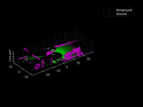
This example employs a hybrid approach that uses the segmentGroundFromLidarData and pcfitplane functions. First, estimate the ground plane parameters using the segmentGroundFromLidarData function. The estimated ground plane is divided into strips along the direction of the vehicle in order to fit the plane, using the pcfitplane function on each strip. This hybrid approach robustly fits the ground plane in a piecewise manner and handles variations in the point cloud.

% Load point cloud
ptCloud = ptClouds{1};
% Define ROI for cropping point cloud
xLimit = [-30,30];
yLimit = [-12,12];
zLimit = [-3,15];

roi = [xLimit,yLimit,zLimit];
% Extract ground plane
[nonGround,ground] = helperExtractGround(ptCloud,roi);
figure;
pcshowpair(nonGround,ground);
axis on;
legend({'\color{white} Nonground','\color{white} Ground'},'Location','northeastoutside');

$Figure contains an axes object. The axes object contains 2 objects of type scatter. These objects represent \color{white} Nonground, \color{white} Ground.$

Semantic Segmentation

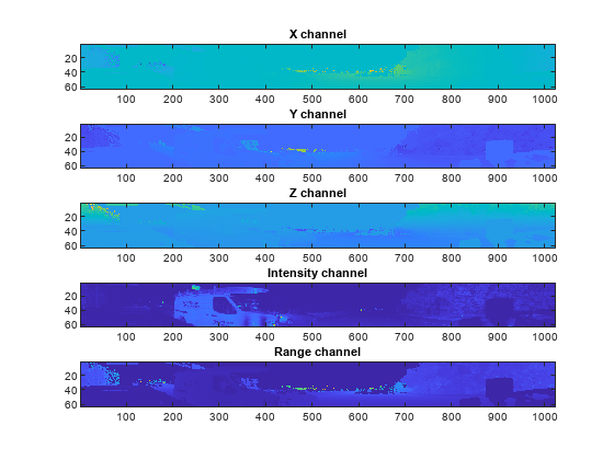
This example uses a pretrained PointSeg network model. PointSeg is an end-to-end real-time semantic segmentation network trained for object classes like cars, trucks, and background. The output from the network is a masked image with each pixel labeled per its class. This mask is used to filter different types of objects in the point cloud. The input to the network is five-channel image, that is x, y, z, intensity, and range. For more information on the network or how to train the network, refer to the Lidar Point Cloud Semantic Segmentation Using PointSeg Deep Learning Network example.

Prepare Input Data

The helperPrepareData function generates five-channel data from the loaded point cloud data.

% Load and visualize a sample frame
frame = helperPrepareData(ptCloud);
figure;
subplot(5,1,1);
imagesc(frame(:,:,1));
title('X channel');

subplot(5,1,2);
imagesc(frame(:,:,2));
title('Y channel');

subplot(5,1,3);
imagesc(frame(:,:,3));
title('Z channel');

subplot(5,1,4);
imagesc(frame(:,:,4));
title('Intensity channel');

subplot(5,1,5);
imagesc(frame(:,:,5));
title('Range channel');

Figure contains 5 axes objects. Axes object 1 with title X channel contains an object of type image. Axes object 2 with title Y channel contains an object of type image. Axes object 3 with title Z channel contains an object of type image. Axes object 4 with title Intensity channel contains an object of type image. Axes object 5 with title Range channel contains an object of type image.

Run forward inference on one frame from the loaded pre-trained network.

if ~exist('net','var')
    net = pretrainedModel.net;
end

% Define classes
classes = ["background","car","truck"];

% Define color map
lidarColorMap = [
            0.98  0.98   0.00  % unknown
            0.01  0.98   0.01  % green color for car
            0.01  0.01   0.98  % blue color for motorcycle
            ];

% Run forward pass
pxdsResults = semanticseg(frame,net);

% Overlay intensity image with segmented output
segmentedImage = labeloverlay(uint8(frame(:,:,4)),pxdsResults,'Colormap',lidarColorMap,'Transparency',0.5);

% Display results
figure;
imshow(segmentedImage);
helperPixelLabelColorbar(lidarColorMap,classes);

Figure contains an axes object. The axes object contains an object of type image.

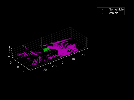
Use the generated semantic mask to filter point clouds containing trucks. Similarly, filter point clouds for other classes.

truckIndices = pxdsResults == 'truck';
truckPointCloud = select(nonGround,truckIndices,'OutputSize','full');

% Crop point cloud for better display
croppedPtCloud = select(ptCloud,findPointsInROI(ptCloud,roi));
croppedTruckPtCloud = select(truckPointCloud,findPointsInROI(truckPointCloud,roi));

% Display ground and nonground points
figure;
pcshowpair(croppedPtCloud,croppedTruckPtCloud);
axis on;
legend({'\color{white} Nonvehicle','\color{white} Vehicle'},'Location','northeastoutside');

$Figure contains an axes object. The axes object contains 2 objects of type scatter. These objects represent \color{white} Nonvehicle, \color{white} Vehicle.$

Clustering and Bounding Box Fitting

After extracting point clouds of different object classes, the objects are clustered by applying Euclidean clustering using the pcsegdist function. To group all the points belonging to one single cluster, the point cloud obtained as a cluster is used as seed points for growing region in nonground points. Use the findNearestNeighbors function to loop over all the points to grow the region. The extracted cluster is fitted in an L-shape bounding box using the pcfitcuboid function. These clusters of vehicles resemble the shape of the letter L when seen from a top-down view. This feature helps in estimating the orientation of the vehicle. The oriented bounding box fitting helps in estimating the heading angle of the objects, which is useful in applications such as path planning and traffic maneuvering.

The cuboid boundaries of the clusters can also be calculated by finding the minimum and maximum spatial extents in each direction. However, this method fails in estimating the orientation of the detected vehicles. The difference between the two methods is shown in the figure.

Screenshot from 2020-07-13 12-47-22.png

[labels,numClusters] = pcsegdist(croppedTruckPtCloud,1);

% Define cuboid parameters
params = zeros(0,9);

for clusterIndex = 1:numClusters
    ptsInCluster = labels == clusterIndex;
        
    pc = select(croppedTruckPtCloud,ptsInCluster);
    location = pc.Location;
    
    xl = (max(location(:,1)) - min(location(:,1)));
    yl = (max(location(:,2)) - min(location(:,2)));
    zl = (max(location(:,3)) - min(location(:,3)));
    
    % Filter small bounding boxes
    if size(location,1)*size(location,2) > 20 && any(any(pc.Location)) && xl > 1 && yl > 1
        indices = zeros(0,1);
        objectPtCloud = pointCloud(location);        
        for i = 1:size(location,1)
            seedPoint = location(i,:);
            indices(end+1) = findNearestNeighbors(nonGround,seedPoint,1);
        end
        
        % Remove overlapping indices        
        indices = unique(indices);
        
        % Fit oriented bounding box
        model = pcfitcuboid(select(nonGround,indices));
        params(end+1,:) = model.Parameters;
    end
end

% Display point cloud and detected bounding box
figure;
pcshow(croppedPtCloud.Location,croppedPtCloud.Location(:,3));
showShape('cuboid',params,"Color","red","Label","Truck");
axis on;

Figure contains an axes object. The axes object contains an object of type scatter.

Visualization Setup

Use the helperLidarObjectDetectionDisplay class to visualize the complete workflow in one window. The layout of the visualization window is divided into the following sections:

Lidar Range Image: point cloud image in 2-D as a range image
Segmented Image: Detected labels generated from the semantic segmentation network overlaid with the intensity image or the fourth channel of the data
Oriented Bounding Box Detection: 3-D point cloud with oriented bounding boxes
Top View: Top view of the point cloud with oriented bounding boxes

display = helperLidarObjectDetectionDisplay;

Loop Through Data

The helperLidarObjectDetection class is a wrapper encapsulating all the segmentation, clustering, and bounding box fitting steps mentioned in the above sections. Use the findDetections function to extract the detected objects.

% Initialize lidar object detector
lidarDetector = helperLidarObjecDetector('Model',net,'XLimits',xLimit,...
    'YLimit',yLimit,'ZLimit',zLimit);

% Prepare 5-D lidar data
inputData = helperPrepareData(ptClouds);

% Set random number generator for reproducible results
S = rng(2018);

% Initialize the display
initializeDisplay(display);

numFrames = numel(inputData);
for count = 1:numFrames
    
    % Get current data
    input = inputData{count};
    
    rangeImage = input(:,:,5);
    
    % Extact bounding boxes from lidar data
    [boundingBox,coloredPtCloud,pointLabels] = detectBbox(lidarDetector,input);
            
    % Update display with colored point cloud
    updatePointCloud(display,coloredPtCloud);
    
    % Update bounding boxes
    updateBoundingBox(display,boundingBox);
    
    % Update segmented image 
    updateSegmentedImage(display,pointLabels,rangeImage);
    
    drawnow('limitrate');
end

{"String":"Figure Object Detection contains 4 axes objects and other objects of type uipanel. Axes object 1 contains an object of type scatter. Axes object 2 contains an object of type scatter. Axes object 3 contains an object of type image. Axes object 4 contains an object of type image.","Tex":[],"LaTex":[]}

Tracking Oriented Bounding Boxes

In this example, you use a joint probabilistic data association (JPDA) tracker. The time step dt is set to 0.1 seconds since the dataset is captured at 10 Hz. The state-space model used in the tracker is based on a cuboid model with parameters, $[x, y, z, ϕ, l, w, h]$ . For more details on how to track bounding boxes in lidar data, see the Track Vehicles Using Lidar: From Point Cloud to Track List (Sensor Fusion and Tracking Toolbox) example. In this example, the class information is provided using the ObjectAttributes property of the objectDetection object. When creating new tracks, the filter initialization function, defined using the helper function helperMultiClassInitIMMFilter uses the class of the detection to set up initial dimensions of the object. This helps the tracker to adjust bounding box measurement model with the appropriate dimensions of the track.

Set up a JPDA tracker object with these parameters.

assignmentGate = [10 100]; % Assignment threshold;
confThreshold = [7 10];    % Confirmation threshold for history logi
delThreshold = [2 3];     % Deletion threshold for history logic
Kc = 1e-5;                 % False-alarm rate per unit volume

% IMM filter initialization function
filterInitFcn = @helperMultiClassInitIMMFilter;

% A joint probabilistic data association tracker with IMM filter
tracker = trackerJPDA('FilterInitializationFcn',filterInitFcn,...
    'TrackLogic','History',...
    'AssignmentThreshold',assignmentGate,...
    'ClutterDensity',Kc,...
    'ConfirmationThreshold',confThreshold,...
    'DeletionThreshold',delThreshold,'InitializationThreshold',0);

allTracks = struct([]);
time = 0;
dt = 0.1;

% Define Measurement Noise
measNoise = blkdiag(0.25*eye(3),25,eye(3));

numTracks = zeros(numFrames,2);

The detected objects are assembled as a cell array of objectDetection (Automated Driving Toolbox) objects using the helperAssembleDetections function.

display = helperLidarObjectDetectionDisplay;
initializeDisplay(display);

for count = 1:numFrames
    time = time + dt;
    % Get current data
    input = inputData{count};
    
    rangeImage = input(:,:,5);
    
    % Extact bounding boxes from lidar data
    [boundingBox,coloredPtCloud,pointLabels] = detectBbox(lidarDetector,input);
    
    % Assemble bounding boxes into objectDetections
    detections = helperAssembleDetections(boundingBox,measNoise,time);
    
    % Pass detections to tracker
    if ~isempty(detections)
        % Update the tracker
         [confirmedTracks,tentativeTracks,allTracks,info] = tracker(detections,time);
         numTracks(count,1) = numel(confirmedTracks);
    end
    
    % Update display with colored point cloud
    updatePointCloud(display,coloredPtCloud);
            
    % Update segmented image 
    updateSegmentedImage(display,pointLabels,rangeImage);
    
    % Update the display if the tracks are not empty
     if ~isempty(confirmedTracks)
        updateTracks(display,confirmedTracks);
     end
     
    drawnow('limitrate');
end

Summary

This example showed how to detect and classify vehicles fitted with oriented bounding box on lidar data. You also learned how to use IMM filter to track objects with multiple class information. The semantic segmentation results can be improved further by adding more training data.

Supporting Functions

helperPrepareData

function multiChannelData = helperPrepareData(input)
% Create 5-channel data as x, y, z, intensity and range
% of size 64-by-1024-by-5 from pointCloud.

if isa(input, 'cell')
    numFrames = numel(input);
    multiChannelData = cell(1, numFrames);
    for i = 1:numFrames
        inputData = input{i};
        
        x = inputData.Location(:,:,1);
        y = inputData.Location(:,:,2);
        z = inputData.Location(:,:,3);
        
        intensity = inputData.Intensity;
        range = sqrt(x.^2 + y.^2 + z.^2);
        
        multiChannelData{i} = cat(3, x, y, z, intensity, range);
    end
else
    x = input.Location(:,:,1);
    y = input.Location(:,:,2);
    z = input.Location(:,:,3);
    
    intensity = input.Intensity;
    range = sqrt(x.^2 + y.^2 + z.^2);
    
    multiChannelData = cat(3, x, y, z, intensity, range);
end
end

pixelLabelColorbar

function helperPixelLabelColorbar(cmap, classNames)
% Add a colorbar to the current axis. The colorbar is formatted
% to display the class names with the color.

colormap(gca,cmap)

% Add colorbar to current figure.
c = colorbar('peer', gca);

% Use class names for tick marks.
c.TickLabels = classNames;
numClasses = size(cmap,1);

% Center tick labels.
c.Ticks = 1/(numClasses*2):1/numClasses:1;

% Remove tick mark.
c.TickLength = 0;
end

helperExtractGround

function [ptCloudNonGround,ptCloudGround] = helperExtractGround(ptCloudIn,roi)
% Crop the point cloud

idx = findPointsInROI(ptCloudIn,roi);
pc = select(ptCloudIn,idx,'OutputSize','full');

% Get the ground plane the indices using piecewise plane fitting
[ptCloudGround,idx] = piecewisePlaneFitting(pc,roi);

nonGroundIdx = true(size(pc.Location,[1,2]));
nonGroundIdx(idx) = false;
ptCloudNonGround = select(pc,nonGroundIdx,'OutputSize','full');
end


function [groundPlane,idx] = piecewisePlaneFitting(ptCloudIn,roi)
groundPtsIdx = ...
    segmentGroundFromLidarData(ptCloudIn, ...
    'ElevationAngleDelta',5,'InitialElevationAngle',15);
groundPC = select(ptCloudIn,groundPtsIdx,'OutputSize','full');

% Divide x-axis in 3 regions
segmentLength = (roi(2) - roi(1))/3;

x1 = [roi(1),roi(1) + segmentLength];
x2 = [x1(2),x1(2) + segmentLength];
x3 = [x2(2),x2(2) + segmentLength];

roi1 = [x1,roi(3:end)];
roi2 = [x2,roi(3:end)];
roi3 = [x3,roi(3:end)];

idxBack = findPointsInROI(groundPC,roi1);
idxCenter = findPointsInROI(groundPC,roi2);
idxForward = findPointsInROI(groundPC,roi3);

% Break the point clouds in front and back
ptBack = select(groundPC,idxBack,'OutputSize','full');

ptForward = select(groundPC,idxForward,'OutputSize','full');

[~,inliersForward] = planeFit(ptForward);
[~,inliersBack] = planeFit(ptBack);
idx = [inliersForward; idxCenter; inliersBack];
groundPlane = select(ptCloudIn, idx,'OutputSize','full');
end

function [plane,inlinersIdx] = planeFit(ptCloudIn)
[~,inlinersIdx, ~] = pcfitplane(ptCloudIn,1,[0, 0, 1]);
plane = select(ptCloudIn,inlinersIdx,'OutputSize','full');
end

helperAssembleDetections

function mydetections = helperAssembleDetections(bboxes,measNoise,timestamp)
% Assemble bounding boxes as cell array of objectDetection

mydetections = cell(size(bboxes,1),1);
for i = 1:size(bboxes,1)
    classid = bboxes(i,end);
    lidarModel = [bboxes(i,1:3), bboxes(i,end-1), bboxes(i,4:6)];
    % To avoid direct confirmation by the tracker, the ClassID is passed as
    % ObjectAttributes.
    mydetections{i} = objectDetection(timestamp, ...
        lidarModel','MeasurementNoise',...
        measNoise,'ObjectAttributes',struct('ClassID',classid));
end
end

helperDownloadData

function [lidarData, pretrainedModel] = helperDownloadData
outputFolder = fullfile(tempdir,'WPI');
url = 'https://ssd.mathworks.com/supportfiles/lidar/data/lidarSegmentationAndTrackingData.tar.gz';
lidarDataTarFile = fullfile(outputFolder,'lidarSegmentationAndTrackingData.tar.gz');
if ~exist(lidarDataTarFile,'file')
    mkdir(outputFolder);
    websave(lidarDataTarFile,url);
    untar(lidarDataTarFile,outputFolder);
end
% Check if tar.gz file is downloaded, but not uncompressed
if ~exist(fullfile(outputFolder,'highwayData.mat'),'file')
    untar(lidarDataTarFile,outputFolder);
end
% Load lidar data
data = load(fullfile(outputFolder,'highwayData.mat'));
lidarData = data.ptCloudData;

% Download pretrained model
url = 'https://ssd.mathworks.com/supportfiles/lidar/data/pretrainedPointSegModel.mat';
modelFile = fullfile(outputFolder,'pretrainedPointSegModel.mat');
if ~exist(modelFile,'file')
    websave(modelFile,url);
end
pretrainedModel = load(fullfile(outputFolder,'pretrainedPointSegModel.mat'));
end

References

[1] Xiao Zhang, Wenda Xu, Chiyu Dong and John M. Dolan, "Efficient L-Shape Fitting for Vehicle Detection Using Laser Scanners", IEEE Intelligent Vehicles Symposium, June 2017

[2] Y. Wang, T. Shi, P. Yun, L. Tai, and M. Liu, “Pointseg: Real-time semantic segmentation based on 3d lidar point cloud,” arXiv preprint arXiv:1807.06288, 2018.

References

[1] WPI Lidar Visual SLAM Dataset, GitHub repository, accessed August 29, 2024, https://github.com/WPI-APA-Lab/WPI-Lidar-Visual-SLAM-Dataset.