Fuzzy ODE Model of SI Engine Torque Dynamics

Since R2026a

This example shows how to use fuzzy ordinary differential equation (FODE) [1] to model the nonlinear torque dynamics of a spark-ignition (SI) engine. The FODE model is trained using the system input and output measurements to identify the model. This example uses the measurements described in the Neural State-Space Model of SI Engine Torque Dynamics (System Identification Toolbox) example.

Load and Preprocess Data

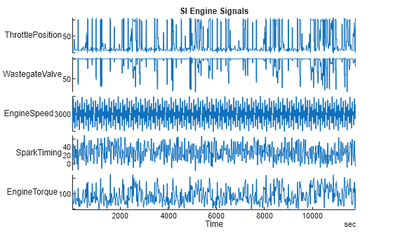
The Neural State-Space Model of SI Engine Torque Dynamics (System Identification Toolbox) example includes a timetable data set with over 100,000 data points sampled at 10 Hz. For this example, you use a dataset that has been downsampled by a factor of 10. Therefore, the timetable contains over 10,000 observations of the following five variables measured at 1 Hz.

Throttle position (degrees)
Wastegate valve area (aperture percentage)
Engine speed (RPM)
Spark timing (degrees)
Engine torque (Nm)

Load and display the engine data timetable.

load FODESIEngineData IOData
stackedplot(IOData)
title("SI Engine Signals")

Figure contains an object of type stackedplot. The chart of type stackedplot has title SI Engine Signals.

The FODE training objective is to generate a dynamic system that outputs the derivative of the engine torque based on the current values of the engine torque and the other four input variables.

The data from the original example is in a single timetable. For this example, you:

Normalize the data, which helps keep input variables within the defined range of their respective FIS inputs.
Extract the data time step value ts.
Split the data into training (first 6,000 data points) and validation (remaining data points) portions.
Extract input and output data arrays for training, uTrain and xTrain, respectively.
Extract input and output data arrays for validation, uVal and xVal, respectively.

To do so, use the preprocessData helper function included at the end of this example.

[uTrain,xTrain,uVal,xVal,ts] = preprocessData(IOData);

FODE Model

The state trajectory in a FODE model is:

$x_{k + 1} = x_{k} + d (z_{k}; θ),$

where:

$x_{k}$ contains the state values at time step $k$ .
$d = (d_{1}, \dots, d_{n_{x}})$ approximates state derivatives using fuzzy inference systems (FISs), where $n_{x}$ is the number of states. You can use a multiple-input, multiple-output FIS to approximate all the state derivatives, or you can use a separate multiple-input, single-output FIS to approximate individual state derivatives.
$z_{k} = {(x_{1, k}, \dots, x_{n_{x}, k}, u_{1, k}, \dots, u_{n_{u}, k})}^{T}$ is the FIS input vector, which concatenates both states and inputs at time step $k$ , where $u$ is a system input and $n_{u}$ is the number of inputs.
$θ$ contains the learning parameters of a FIS.

For the SI engine model:

There are four inputs ( $n_{u} = 4$ ).
Engine torque is modeled both as a state ( $n_{x} = 1$ ) and an output.

Format Data for FIS Tuning

Since the output measurement is available, you can calculate the state difference and learn the FIS parameters as follows:

$d (z_{k}; θ) = x_{k + 1} - x_{k}$

Calculate the actual state difference from the output training data. This state difference vector is the output data for tuning the FIS parameters.

xDiff = diff(xTrain);

Create the input data for tuning the FIS parameters. This array contains the current engine torque value along with the other four input variables.

zTrain = [xTrain(1:end-1) uTrain(1:end-1,:)];

Create Initial FIS

Create an initial FIS based on the training data using the genfis function.

Use the subtractive clustering method and specify 10 random initial cluster centers. For reproducibility, use default random number generator settings.

rng("default")
options = genfisOptions("SubtractiveClustering");
options.CustomClusterCenters = rand(10,6);

Generate the initial FIS.

inFIS = genfis(zTrain,xDiff,options);
inFIS.Inputs(1).Name = "engineTorque";
inFIS.Inputs(2).Name = "throttlePosition";
inFIS.Inputs(3).Name = "wastegateValveArea";
inFIS.Inputs(4).Name = "engineSpeed";
inFIS.Inputs(5).Name = "spark timing";
inFIS.Outputs(1).Name = "dEngineTorque";

The generated FIS is a type-1 Sugeno system.

Tune FIS Parameters

Optimize the input and output membership function (MF) parameters of the initial FIS using the tunefis function.

Specify the tuning options. Use the ANFIS tuning method and set the maximum number of training epochs to 100.

options = tunefisOptions(Method="anfis",Display="none");
options.MethodOptions.EpochNumber = 100;

Tune the MF parameters.

[inpset,outpset] = getTunableSettings(inFIS);
[outFIS,info] = tunefis(inFIS,[inpset;outpset],zTrain,xDiff,options);

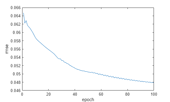
Plot the root mean squared error for each training epoch.

figure
plot(info.tuningOutputs.trainError)
xlabel("epoch")
ylabel("rmse")

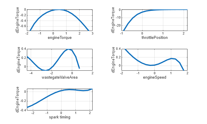
Figure contains an axes object. The axes object with xlabel epoch, ylabel rmse contains an object of type line.

View control surface plots of the input-output mappings of the tuned FIS. These plots show the impact of each input variable on the difference output while keeping the other input values fixed to their mid-range values.

h = figure;
h.Position(3) = 1.25*h.Position(3);
h.Position(4) = 1.25*h.Position(4);
tiledlayout(3,2)
nexttile
gensurf(outFIS,gensurfOptions(InputIndex=1))
nexttile
gensurf(outFIS,gensurfOptions(InputIndex=2))
nexttile
gensurf(outFIS,gensurfOptions(InputIndex=3))
nexttile
gensurf(outFIS,gensurfOptions(InputIndex=4))
nexttile
gensurf(outFIS,gensurfOptions(InputIndex=5))

Predict State Trajectory Using Training Data

Predict the state trajectory using the input values from the training data. To do so, use the predictState helper function included at the end of this example. At each time step, this function computes the engine torque difference using the tuned FIS and predicts the engine torque for the next time step by adding the predicted difference to the current engine torque.

[xPred,accuracy] = predictState(xTrain,uTrain,outFIS);

The predictState function returns the predicted state trajectory and the normalized root mean squared accuracy.

accuracy

accuracy = 
91.6188

When using the training data, the predicted state trajectory is about 92% accurate.

Qualitatively confirm the accuracy by viewing the predicted and actual state trajectories. To do so, use the plotStateTrajectories helper function included at the end of this example.

plotStateTrajectories(xTrain,xPred,accuracy,ts,"Training data")

Figure contains an axes object. The axes object with title State prediction using training data [accuracy = 91.62%], xlabel Runtime (sec), ylabel Torque (N m) contains 2 objects of type line. These objects represent Training data, Prediction.

Predict State Trajectory Using Validation Data

To validate the generalization of the tuned FODE beyond the training data, predict the state trajectory using the validation data.

[xPred,accuracy] = predictState(xVal,uVal,outFIS);
accuracy

accuracy = 
89.3418

In this case, the predicted state trajectory matches the validation data with about 90% accuracy.

Plot the state trajectories.

plotStateTrajectories(xVal,xPred,accuracy,ts,"Validation data")

Figure contains an axes object. The axes object with title State prediction using validation data [accuracy = 89.34%], xlabel Runtime (sec), ylabel Torque (N m) contains 2 objects of type line. These objects represent Validation data, Prediction.

Next Steps

This example uses a type-1 Sugeno FIS for modeling the FODE. To potentially improve results, you can consider one or both of the following modifications:

To improve the explainability of the rule consequents, use a Mamdani FIS.
To model higher levels of uncertainty and potentially obtain an FODE more robust to noise, use an interval type-2 FIS.

In both of these cases, use a tuning method other than the ANFIS method.

References

[1] Yusuf Güven and Tufan Kumbasar. "Fuzzy Logic Strikes Back: Fuzzy ODEs for Dynamic Modeling and Uncertainty Quantification." IEEE Transactions on Artificial Intelligence, early access (2025).

Helper Functions

function [uTrain,xTrain,uVal,xVal,ts] = preprocessData(IOData)

% Normalize the data.
IODataN = normalize(IOData);

% Extract data time step.
ts = seconds(IODataN.Properties.TimeStep);

% Convert timetable to array.
IODataA = table2array(IODataN);

% Split data into training (first 6,000 data points) and validation (remaining data points) portions.
numTrainingPoints = 6000;
trnData = IODataA(1:numTrainingPoints,:);
valData = IODataA(numTrainingPoints+1:end,:);

% Extract input and output training data.
uTrain = trnData(:,1:end-1);
xTrain = trnData(:,end);

% Extract input and output validation data.
uVal = valData(:,1:end-1);
xVal = valData(:,end);

end

function [xPred,accuracy] = predictState(xTrain,uTrain,outFIS)
% Predict state trajectory with RMSE and accuracy.

% Initialize state prediction data.
xPred = zeros(size(xTrain));
xPred(1) = xTrain(1); % Initial state

% Specify options for FIS evaluation.
options = evalfisOptions(...
    OutOfRangeInputValueMessage="none", ...
    NoRuleFiredMessage="none", ...
    EmptyOutputFuzzySetMessage="none");

% Predict state.
for ct = 1:size(uTrain,1)-1
    d = evalfis(outFIS,[xPred(ct) uTrain(ct,:)],options);
    xPred(ct+1) = xPred(ct) + d;
end

% Calculate prediction accuracy.
nrmse = sqrt(sum((xPred-xTrain).^2)./sum((xTrain-mean(xTrain)).^2)); 
accuracy = 100*(1-nrmse);

end

function plotStateTrajectories(xTrain,xPred,accuracy,ts,dataType)
% Plot reference and predicted state trajectories

t = 0:ts:ts*(length(xPred)-1);
figure
plot(t,[xTrain xPred])
legend([dataType "Prediction"])
titleStr = sprintf("State prediction using %s [accuracy = %2.2f%%]", ...
    lower(dataType),accuracy);
title(titleStr)
xlabel("Runtime (sec)")
ylabel("Torque (N m)")
end