Constrained Minimization Using the Genetic Algorithm

Constrained Minimization Problem

For this problem, the objective function to minimize is a simple function of a 2-D variable x.

simple_objective(x) = (4 - 2.1*x(1)^2 + x(1)^4/3)*x(1)^2 + x(1)*x(2) + (-4 + 4*x(2)^2)*x(2)^2;

This function is known as "cam," as described in L.C.W. Dixon and G.P. Szego [1].

Additionally, the problem has nonlinear constraints and bounds.

   x(1)*x(2) + x(1) - x(2) + 1.5 <= 0  (nonlinear constraint)
   10 - x(1)*x(2) <= 0                 (nonlinear constraint)
   0 <= x(1) <= 1                      (bound)
   0 <= x(2) <= 13                     (bound)

Code the Fitness Function

Create a MATLAB file named simple_objective.m containing the following code:

type simple_objective

function y = simple_objective(x)
%SIMPLE_OBJECTIVE Objective function for PATTERNSEARCH solver

%   Copyright 2004 The MathWorks, Inc.  

x1 = x(1);
x2 = x(2);
y = (4-2.1.*x1.^2+x1.^4./3).*x1.^2+x1.*x2+(-4+4.*x2.^2).*x2.^2;

Solvers such as ga accept a single input x, where x has as many elements as the number of variables in the problem. The objective function computes the scalar value of the objective function and returns it in its single output argument y.

Code the Constraint Function

Create a MATLAB file named simple_constraint.m containing the following code:

type simple_constraint

function [c, ceq] = simple_constraint(x)
%SIMPLE_CONSTRAINT Nonlinear inequality constraints.

%   Copyright 2005-2007 The MathWorks, Inc.

c = [1.5 + x(1)*x(2) + x(1) - x(2); 
     -x(1)*x(2) + 10];

% No nonlinear equality constraints:
ceq = [];

The constraint function computes the values of all the inequality and equality constraints and returns the vectors c and ceq, respectively. The value of c represents nonlinear inequality constraints that the solver attempts to make less than or equal to zero. The value of ceq represents nonlinear equality constraints that the solver attempts to make equal to zero. This example has no nonlinear equality constraints, so ceq = []. For details, see Nonlinear Constraints.

Minimizing Using ga

Specify the objective function as a function handle.

ObjectiveFunction = @simple_objective;

Specify the problem bounds.

lb = [0 0];   % Lower bounds
ub = [1 13];  % Upper bounds

Specify the nonlinear constraint function as a function handle.

ConstraintFunction = @simple_constraint;

Specify the number of problem variables.

nvars = 2;

Call the solver, requesting the optimal point x and the function value at the optimal point fval.

rng default % For reproducibility
[x,fval] = ga(ObjectiveFunction,nvars,[],[],[],[],lb,ub,ConstraintFunction)

Optimization finished: average change in the fitness value less than options.FunctionTolerance and constraint violation is less than options.ConstraintTolerance.

x = 1×2

    0.8122   12.3103

fval = 
9.1268e+04

Add Visualization

To observe the solver's progress, specify options that select two plot functions. The plot function gaplotbestf plots the best objective function value at every iteration, and the plot function gaplotmaxconstr plots the maximum constraint violation at every iteration. Set these two plot functions in a cell array. Also, display information about the solver's progress in the Command Window by setting the Display option to 'iter'.

options = optimoptions("ga",'PlotFcn',{@gaplotbestf,@gaplotmaxconstr}, ...
    'Display','iter');

Run the solver, including the options argument.

[x,fval] = ga(ObjectiveFunction,nvars,[],[],[],[],lb,ub, ...
    ConstraintFunction,options)

Single objective optimization:
2 Variables
2 Nonlinear inequality constraints

Options:
CreationFcn:       @gacreationuniform
CrossoverFcn:      @crossoverscattered
SelectionFcn:      @selectionstochunif
MutationFcn:       @mutationadaptfeasible

                              Best       Max        Stall
Generation  Func-count        f(x)     Constraint  Generations
    1           2524       91986.8    7.796e-09      0
    2           4986       94678.2            0      0
    3          10362       96473.7            0      0
    4          16243       91270.1    0.0009897      0
Optimization finished: average change in the fitness value less than options.FunctionTolerance and constraint violation is less than options.ConstraintTolerance.

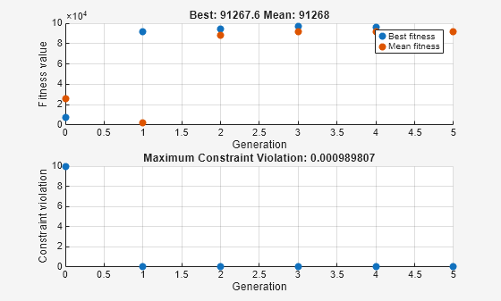
x = 1×2

    0.8123   12.3104

fval = 
9.1270e+04

With iterative display, that ga provides details about the problem type and the creation, crossover, mutation, and selection operators.

Nonlinear constraints cause ga to solve many subproblems at each iteration. As shown in both the plots and the iterative display, the solution process has few iterations. However, the Func-count column in the iterative display shows many function evaluations per iteration.

The ga solver handles linear constraints and bounds differently from nonlinear constraints. All the linear constraints and bounds are satisfied throughout the optimization. However, ga may not satisfy all the nonlinear constraints at every generation. If ga converges to a solution, the nonlinear constraints will be satisfied at that solution.

ga uses the mutation and crossover functions to produce new individuals at every generation. The way the ga satisfies the linear and bound constraints is to use mutation and crossover functions that only generate feasible points. For example, in the previous call to ga, the default mutation function (for unconstrained problems) mutationgaussian does not satisfy the linear constraints and so ga uses the mutationadaptfeasible function instead by default. If you provide a custom mutation function, this custom function must only generate points that are feasible with respect to the linear and bound constraints. All the crossover functions in the toolbox generate points that satisfy the linear constraints and bounds.

However, when your problem contains integer constraints, ga enforces that all iterations satisfy bounds and linear constraints. This feasibility occurs for all mutation, crossover, and creation operators, to within a small tolerance.

Provide a Start Point

To speed the solver, you can provide an initial population in the InitialPopulationMatrix option. ga uses the initial population to start its optimization. Specify a row vector or a matrix where each row represents one start point.

X0 = [0.8 12.5]; % Start point (row vector)
options.InitialPopulationMatrix = X0;
[x,fval] = ga(ObjectiveFunction,nvars,[],[],[],[],lb,ub, ...
    ConstraintFunction,options)

Single objective optimization:
2 Variables
2 Nonlinear inequality constraints

Options:
CreationFcn:       @gacreationuniform
CrossoverFcn:      @crossoverscattered
SelectionFcn:      @selectionstochunif
MutationFcn:       @mutationadaptfeasible

                              Best       Max        Stall
Generation  Func-count        f(x)     Constraint  Generations
    1           2500       91769.6            0      0
    2           4962       97536.4            0      0
    3           7412       91268.4      0.00098      0
    4           9862       91268.1    0.0009893      0
    5          12312       91267.9    0.0009943      0
Optimization finished: average change in the fitness value less than options.FunctionTolerance and constraint violation is less than options.ConstraintTolerance.

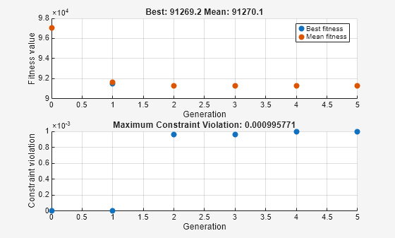
x = 1×2

    0.8122   12.3103

fval = 
9.1268e+04

In this case, providing a start point does not substantially change the solver progress.

References

[1] Dixon, L. C. W., and G .P. Szego (eds.). Towards Global Optimisation 2. North-Holland: Elsevier Science Ltd., Amsterdam, 1978.