Optimize Simulink Model in Parallel with Optimization Explorer

Vectorized Objective Function Based on Simulink Model

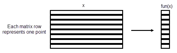
To optimize a Simulink model in parallel, write a vectorized objective function that:

This figure shows how a vectorized objective function works with a matrix of input values, giving a column vector of output values.

For this example, use the Lorenz_system.slx Simulink model.

The objective function is to minimize the sum of squares of the difference between the Lorenz system and the uniform circular motion over a set of times from 0 through 1/10. For times xdata, the objective function is

objective = sum((fitlorenzfn(x,xdata) - lorenz(xdata)).^2) - (F(1) + F(end))/2

where:

Enter the data for the uniform circular motion.

x = zeros(8,1);
x(1) = 1.2814;
x(2) = -1.4930;
x(3) = 24.9763;
x(4) = 14.1870;
x(5) = 0.0545;
x(6:8) = [13.8061;1.5475;25.3616];

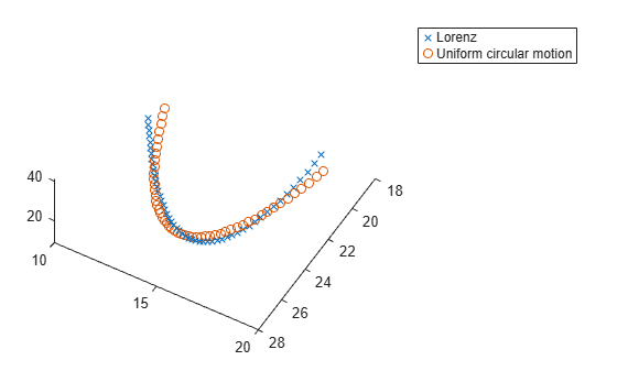
Load the Lorenz system and simulate it with the base parameters. Create a 3-D plot of the resulting system and compare the plot with the specified uniform circular motion.

model = "Lorenz_system";
open_system(model);
in = Simulink.SimulationInput(model);
% params [X0,Y0,Z0,Sigma,Beta,Rho]
params = [10,20,10,10,8/3,28]; % Original parameters Sigma, Beta, Rho
in = setparams(in,model,params);
out = sim(in);
yout = out.yout;
tlist = yout{1}.Values.Time;
YDATA = fitlorenzfn(x,tlist);

figure;
plot3(yout{1}.Values.Data,yout{2}.Values.Data,yout{3}.Values.Data,"x");
view([-30 -70])
hold on
plot3(YDATA(:,1),YDATA(:,2),YDATA(:,3),"o")
legend("Lorenz","Uniform circular motion")
hold off

The parobjfun helper function shown below accepts a matrix of parameters, where each row of the matrix represents one set of parameters. The function calls the setparams helper function (shown at the end of this example) to set parameters for a Simulink.SimulationInput vector. The parobjfun function then calls parsim to evaluate the model on the parameters in parallel. The parobjfun function:

function f = parobjfun(params,YDATA,model)

N = size(params,1);
simIn(1:N) = Simulink.SimulationInput(model);
f = zeros(N,1);
for i = 1:N
    simIn(i) = setparams(simIn(i),model,params(i,:));
end

simOut = parsim(simIn,ShowProgress="off", ...
    UseFastRestart="on");

for i = 1:N
    yout = simOut(i).yout;
    vals = [yout{1}.Values.Data,yout{2}.Values.Data,yout{3}.Values.Data];
    g = sum((YDATA - vals).^2,2);
    f(i) = sum(g) - (g(1) + g(end))/2;
end
end

Set bounds for solvers 20% above and below the current parameter values.

lb = 0.8*params;
ub = 1.2*params;

For added speed, set the simulation to use fast restart.

set_param(model,FastRestart="on");

Define a function to close the model using the closeModel helper function (shown at the end of this example).

c = onCleanup(@()closeModel(model));

For reproducibility, set the random stream.

rng(1)

Define the objective function as parobjfun with its extra parameters.

fitobjective = @(params)parobjfun(params,YDATA,model);

Vectorized Objective Function in Optimization Explorer

Start Optimization Explorer by entering the following at the command line:

optimizationExplorer

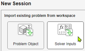
Because you need to use vectorized function evaluations, specify the problem using Solver Inputs.

For the Objective function, select fitobjective. Click Advanced and select Is vectorized. You can leave the Solver selection at the default setting; you specify solvers in the next section.

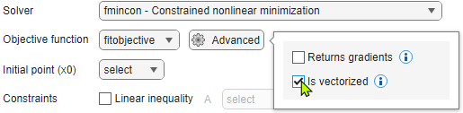
For this problem, choose params as the Initial point (x0) value. For the Constraints, select Bounds and set the bounds lb and ub to lb and ub, respectively. Click Next to continue.

Manually Schedule Solver Configurations

To optimize a Simulink model in parallel, you must run manual configurations, not auto configurations. Therefore, you do not need to select any of the problem attributes such as Convex, Nonsmooth, Expensive, or Simulation. Click Next to continue.

Specify to run Optimization Explorer in Manual mode.

Click Start Session.

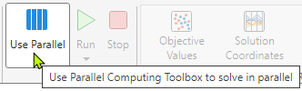
Leave Parallel Off

Although you will run Simulink in parallel in Optimization Explorer, do not use the app's default parallel mode. The Use Parallel button is not appropriate for optimizing a Simulink model.

Choose Solvers and Options

To schedule solver configurations, you use the Select Solvers section of the toolstrip. After you select a solver, the app opens a tab with options for that solver. Begin by selecting the ga solver.

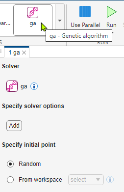
Use the Add button to display solver options you can set. For some solvers, such as patternsearch, you first need to select the algorithm for the solver. To set additional options, click the plus sign that appears to the right of an option you set.

Schedule these solver algorithms, all of which can run in a vectorized manner: ga, patternsearch (nups), patternsearch (classic), surrogateopt, and particleswarm. To run the example reasonably quickly, set the maximum number of function evaluations to 300 for each solver (for ga and particleswarm, have a population of 12 run for 25 iterations). Set the following options:

        Note: To run patternsearch (classic) in a vectorized manner, you must use a complete poll.

   4. Specify initial point: From workspace > params

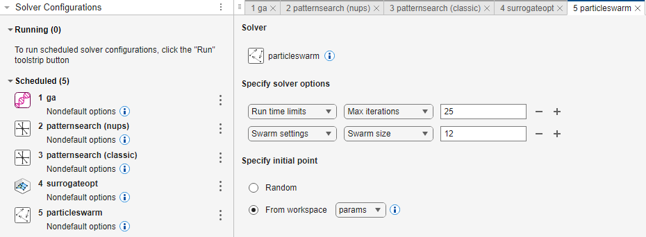
After making the solver selections, run Optimization Explorer by clicking the Run button on the toolstrip. The Solver Configurations panel shows which solver is running and which solvers are scheduled to run.

Results

After Optimization Explorer finishes, you see the following or similar results.

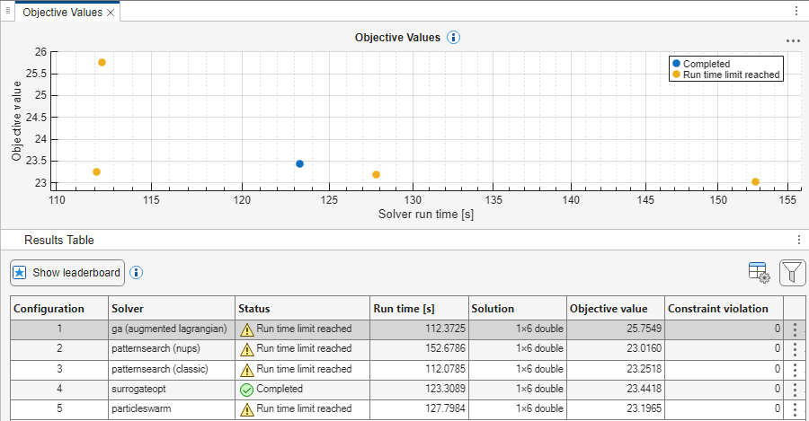
As shown in these results:

Helper Functions

This code creates the fitlorenzfn helper function.

function f = fitlorenzfn(x,xdata)
% Lorenz function
theta = x(1:2);
R = x(3);
V = x(4);
t0 = x(5);
delta = x(6:8);
f = zeros(length(xdata),3);
f(:,3) = R*sin(theta(1))*sin(V*(xdata - t0)) + delta(3);
f(:,1) = R*cos(V*(xdata - t0))*cos(theta(2)) ...
    - R*sin(V*(xdata - t0))*cos(theta(1))*sin(theta(2)) + delta(1);
f(:,2) = R*sin(V*(xdata - t0))*cos(theta(1))*cos(theta(2)) ...
    - R*cos(V*(xdata - t0))*sin(theta(2)) + delta(2);
end

This code creates the setparams helper function.

function pp = setparams(in,model,params)
% parameters [X0,Y0,Z0,Sigma,Beta,Rho]
pp = in.setVariable("X0",params(1),"Workspace",model);
pp = pp.setVariable("Y0",params(2),"Workspace",model);
pp = pp.setVariable("Z0",params(3),"Workspace",model);
pp = pp.setVariable("Sigma",params(4),"Workspace",model);
pp = pp.setVariable("Beta",params(5),"Workspace",model);
pp = pp.setVariable("Rho",params(6),"Workspace",model);
end

This code creates the closeModel helper function. To close the model, you must first disable fast restart.

function closeModel(model)
set_param(model,FastRestart="off");
close_system(model)
end