并行优化 Simulink 模型
此示例展示如何使用多个 Global Optimization Toolbox 求解器并行优化 Simulink® 模型。该示例使用内部调用 parsim 来执行并行计算的矢量化计算。
模型与目标函数
洛仑兹方程组是常微分方程组(请参阅洛仑兹方程组)。对于实常数 和 ,系统为
洛伦兹对敏感系统的参数的取值为 和 。从 [x(0),y(0),z(0)] = [10,20,10] 开始启动系统,查看系统从时间 0 到 100 的演变。
sigma = 10;
beta = 8/3;
rho = 28;
f = @(t,a) [-sigma*a(1) + sigma*a(2); rho*a(1) - a(2) - a(1)*a(3); -beta*a(3) + a(1)*a(2)];
xt0 = [10,20,10];
[tspan,a] = ode45(f,[0 100],xt0);     % Runge-Kutta 4th/5th order ODE solver
figure
plot3(a(:,1),a(:,2),a(:,3))
view([-10.0 -2.0])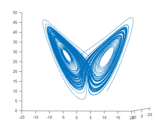
演变相当复杂。但在很短的时间间隔内,该系统看起来有点像匀速圆周运动。绘制 [0,1/10] 时间区间内的解。
[tspan,a] = ode45(f,[0 1/10],xt0);     % Runge-Kutta 4th/5th order ODE solver
figure
plot3(a(:,1),a(:,2),a(:,3))
view([-30 -70])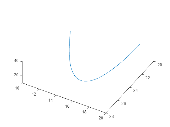
匀速圆周运动依赖于几个参数:
路径与 x-y 平面间的夹角
平面沿 x 轴倾斜的角度
速度
半径
时间偏移
三维偏移
有关这些参数与匀速圆周运动的关系以及将它们拟合到洛伦兹系统的详细信息,请参阅示例拟合常微分方程 (ODE)。
目标函数是最小化从 0 到 1/10 的一组时间内洛伦兹系统和均匀圆周运动之间的差异的平方和。对于时间 xdata,目标函数是
objective = sum((fitlorenzfn(x,xdata) - lorenz(xdata)).^2) - (F(1) + F(end))/2
这里,fitlorenzfn 计算匀速圆周运动路径上的点,lorenz(xdata) 表示 Lorenz 系统在时间 xdata 的 3-D 演变,F 表示圆周和 Lorenz 系统中对应点之间的平方距离矢量。目标是减去端点处的一半值以最好地近似积分。
将匀速圆周运动视为需要拟合的曲线,修改模拟中的 Lorenz 参数,使目标函数最小化。
Simulink 模型
运行此示例时可用的 Lorenz_system.slx 文件实现了 Lorenz 系统。
输入匀速圆周运动的数据。
x = zeros(8,1);
x(1) = 1.2814;
x(2) = -1.4930;
x(3) = 24.9763;
x(4) = 14.1870;
x(5) = 0.0545;
x(6:8) = [13.8061;1.5475;25.3616];
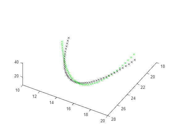
加载 Lorenz 系统并使用基本参数仿真。创建结果系统的 3-D 图并将其与均匀圆周运动进行比较。
model = "Lorenz_system";
open_system(model);
Warning: Unrecognized function or variable 'CloneDetectionUI.internal.CloneDetectionPerspective.register'.
in = Simulink.SimulationInput(model);
% params [X0,Y0,Z0,Sigma,Beta,Rho]
params = [10,20,10, 10,8/3,28]; % The original parameters Sigma, Beta, Rho
in = setparams(in,model,params);
out = sim(in);

yout = out.yout;
h = figure;
plot3(yout{1}.Values.Data,yout{2}.Values.Data,yout{3}.Values.Data,"gx");
view([-30 -70])

tlist = yout{1}.Values.Time;
YDATA = fitlorenzfn(x,tlist);
hold on
plot3(YDATA(:,1),YDATA(:,2),YDATA(:,3),"kx")
hold off
计算绘制时间曲线之间差异的平方和。
ssq = objfun(in,params,YDATA,model)
ssq =
26.9975
并行优化 Simulink 模型参数
正如解释的那样求解器如何并行计算,Global Optimization Toolbox 求解器通常通过内部调用 parfor 或 parfeval 进行并行计算。但是,Simulink 模型不支持这些函数进行并行计算。
为了并行优化 Simulink 模型,请编写一个目标函数:
接受矩阵作为输入,其中矩阵的每一行都是一个参数向量
通过调用
parsim并行执行仿真返回一个值向量,其中向量中的每个条目包含与输入矩阵一行中的参数相对应的目标函数的值
为了使目标函数接受矩阵作为输入,请将求解器的 UseVectorized 选项设置为 true。请勿将 UseParallel 选项设置为 true。您的目标函数必须将参数向量映射到 Simulink 变量,并将 Simulink 结果映射回您的参数。
接下来显示的 parobjfun 辅助函数接受一个参数矩阵,其中矩阵的每一行代表一组参数。该函数调用 setparams 辅助函数(显示在本示例末尾)来设置 Simulink SimulationInput 向量的参数。然后,parobjfun 函数调用 parsim (Simulink) 并行评估模型的参数。
function f = parobjfun(params,YDATA,model)
% Solvers can pass different numbers of points to evaluate.
% N is the number of points on which the simulation must be performed.
N = size(params,1);

% Create a vector of size N simulation inputs for the model.
simIn(1:N) = Simulink.SimulationInput(model);

% Initialize the output.
f = zeros(N,1);

% Map the optimization parameters (params) to each SimulationInput.
for i = 1:N
    simIn(i) = setparams(simIn(i),model,params(i,:));
end

% Set the parsim properties and perform the simulation in parallel.
simOut = parsim(simIn,ShowProgress="off", ...
    UseFastRestart="on");

% Fetch the simulation outputs (a blocking call) and compute the final outputs.
for i = 1:N
    yout = simOut(i).yout;
    vals = [yout{1}.Values.Data,yout{2}.Values.Data,yout{3}.Values.Data];
    g = sum((YDATA - vals).^2,2);
    f(i) = sum(g) - (g(1) + g(end))/2;
end
end
准备匹配均匀圆周运动
如果尚未打开并行池,请打开一个并行池。根据您的并行选项设置,池可以自动打开。为了在第一次并行求解时不计算打开并行池的时间,现在就打开一个。
pool = gcp("nocreate"); % Check whether a parallel pool exists.
if isempty(pool) % If not, create one.
    pool = parpool;
end
将求解器的界限设置为高于和低于当前参数值的 20%。
lb = 0.8*params;
ub = 1.2*params;
为了提高速度,请将模拟设置为使用快速重启。
set_param(model,FastRestart="on");
c = onCleanup(@()closeModel(model));
为了实现可再现性,请设置随机流。
rng(1)
将目标函数定义为 parobjfun 及其额外参数。
fitobjective = @(params)parobjfun(params,YDATA,model);
为了在求解器之间进行公平比较,将每个求解器的最大函数评估次数设置为约 300。
maxf = 300;
patternsearch "nups" 算法
设置 patternsearch "nups" 算法的选项。将 UseVectorized 设置为 true,并设置选项以使用 psplotbestf 和 psplotmeshsize 绘图函数。
options = optimoptions("patternsearch",...
    UseVectorized=true,Algorithm="nups",...
    MaxFunctionEvaluations=maxf,PlotFcn={"psplotbestf" "psplotmeshsize"});
调用求解器并显示平方和与仿真时间的改进。
rng(1)
tic
[fittedparamspsn,fvalpsn] = patternsearch(fitobjective,params,[],[],[],[],lb,ub,[],options);
patternsearch stopped because it exceeded options.MaxFunctionEvaluations.
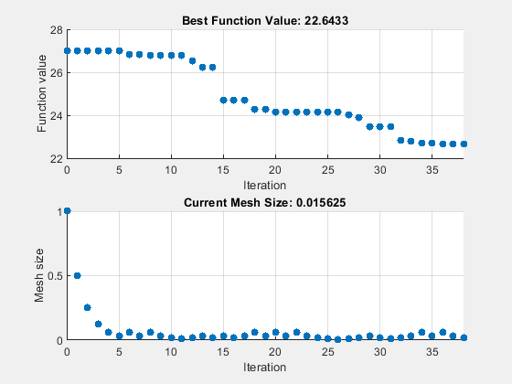
paralleltimepsn = toc
paralleltimepsn =
221.8100
disp([ssq,fvalpsn])
26.9975 22.6433
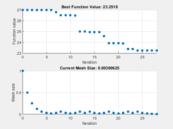
patternsearch "classic" 算法
设置 patternsearch "classic" 算法的选项。将 UseVectorized 设置为 true,并设置选项以使用 psplotbestf 和 psplotmeshsize 绘图函数。要将矢量化与 "classic" 算法一起使用,还必须将 UseCompletePoll 选项设置为 true。
options = optimoptions("patternsearch",...
    UseVectorized=true,UseCompletePoll=true, ...
    Algorithm="classic",...
    MaxFunctionEvaluations=maxf,PlotFcn={"psplotbestf" "psplotmeshsize"});
tic
[fittedparamspsc,fvalpsc] = patternsearch(fitobjective,params,[],[],[],[],lb,ub,[],options);
patternsearch stopped because it exceeded options.MaxFunctionEvaluations.

paralleltimepsc = toc
paralleltimepsc =
147.6369
disp([ssq,fvalpsc])
26.9975 23.2518
遗传算法
设置遗传算法的选项。将 ga 的种群规模设置为正在优化的参数数量的两倍。将起点 params 作为初始种群传递,这样这个相对较好的点就是初始种群的一部分。为了让 ga 评估大约 maxf 个个体,将最大代数设置为 maxf /种群大小。将 UseVectorized 设置为 true。
rng(1)
PopSize = 2*numel(params);
options = optimoptions("ga",PopulationSize=PopSize,...
    UseVectorized=true,InitialPopulationMatrix=params,...
    MaxGenerations=round(maxf/PopSize),PlotFcn="gaplotrange");
tic
[fittedparamsga,fvalga] = ga(fitobjective,numel(params),[],[],[],[],lb,ub,[],options);
ga stopped because it exceeded options.MaxGenerations.
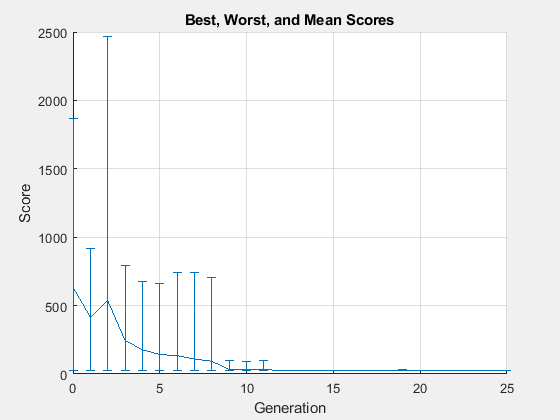
paralleltimega = toc
paralleltimega =
152.9136
disp([ssq,fvalga])
26.9975 24.8405
替代优化
设置替代优化的选项。将 BatchSize 选项设置为正在优化的参数数量的两倍。将函数评估的最大次数设置为批次大小的最大倍数,但不超过 maxf。将 UseVectorized 设置为 true。
rng(1)
BatchSize = 2*numel(params);
myn = floor(maxf/BatchSize)*BatchSize; % Multiple of BatchSize
options = optimoptions("surrogateopt",BatchUpdateInterval=BatchSize,...
    UseVectorized=true,InitialPoints=params,...
    MaxFunctionEvaluations=myn,PlotFcn="optimplotfvalconstr");
tic
[fittedparamssurr,fvalsurr] = surrogateopt(fitobjective,lb,ub,[],[],[],[],[],options);
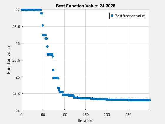
surrogateopt stopped because it exceeded the function evaluation limit set by
'options.MaxFunctionEvaluations'.
paralleltimesur = toc
paralleltimesur =
209.8845
disp([ssq,fvalsurr])
26.9975 24.3026
粒子群优化
设置粒子群优化选项。将群规模设置为正在优化的参数数量的两倍。将最大迭代次数设置为 maxf/群大小。将 UseVectorized 设置为 true。
rng(1)
options = optimoptions("particleswarm",SwarmSize=PopSize,...
    MaxIterations=round(maxf/PopSize),InitialPoints=params,...
    UseVectorized=true,PlotFcn="pswplotbestf");
tic
[fittedparamspsw,fvalpsw] = particleswarm(fitobjective,numel(params),lb,ub,options)
Optimization ended: number of iterations exceeded OPTIONS.MaxIterations.
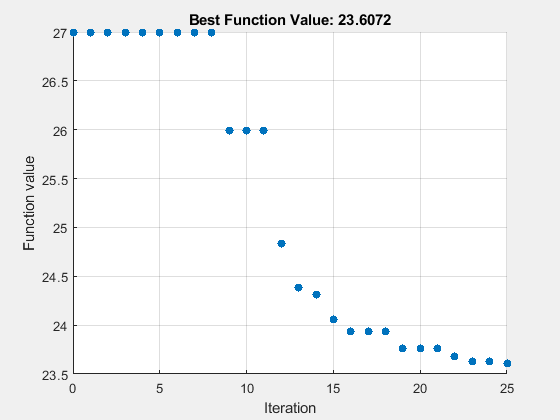
fittedparamspsw = 1×6

   10.4450   19.8899    9.8416    9.4086    2.6612   27.8898
fvalpsw =
23.6072
paralleltimepsw = toc
paralleltimepsw =
274.8291
disp([ssq,fvalpsw])
26.9975 23.6072
与非并行计算比较
为了进行比较,通过将 patternsearch 选项设置为 "classic" 来串行运行 UseVectorized false 算法。
options = optimoptions("patternsearch",...
    UseVectorized=false,UseCompletePoll=true, ...
    Algorithm="classic",...
    MaxFunctionEvaluations=maxf,PlotFcn={"psplotbestf" "psplotmeshsize"});
tic
[fittedparamspscs,fvalpscs] = patternsearch(fitobjective,params,[],[],[],[],lb,ub,[],options);
patternsearch stopped because it exceeded options.MaxFunctionEvaluations.
serialltimepscs = toc
serialltimepscs =
1.4635e+03
disp([ssq,fvalpscs])
26.9975 23.2518
非矢量化(串行)优化比矢量化(并行)优化花费的时间更长,并且达到与并行模式 patternsearch"classic" 算法相同的解。
汇总结果
收集每个求解器的计时结果和最佳函数值。
table(["NUPS";"PSClassic";"ga";"surr";"particleswarm";"PSClassicSerial"],...
    [paralleltimepsn;paralleltimepsc;paralleltimega;paralleltimesur;paralleltimepsw;serialltimepscs], ...
    [fvalpsn;fvalpsc;fvalga;fvalsurr;fvalpsw;fvalpscs],...
    'VariableNames',{'Algorithm' 'Time' 'FVal'})
ans=6×3 table
        Algorithm         Time      FVal
    _________________    ______    ______

    "NUPS"               221.81    22.643
    "PSClassic"          147.64    23.252
    "ga"                 152.91     24.84
    "surr"               209.88    24.303
    "particleswarm"      274.83    23.607
    "PSClassicSerial"    1463.5    23.252
patternsearch "nups" 算法具有最低的目标函数值。绘制该算法的最终轨迹。
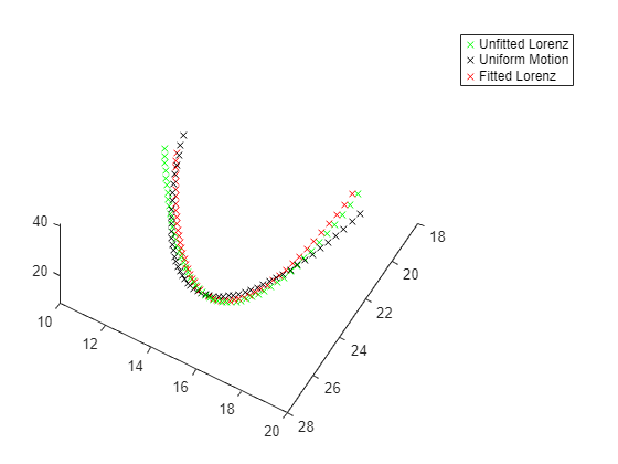
figure(h)
hold on
in = setparams(in,model,fittedparamspsn);
out = sim(in);
yout = out.yout;
plot3(yout{1}.Values.Data,yout{2}.Values.Data,yout{3}.Values.Data,'rx');
legend("Unfitted Lorenz","Uniform Motion","Fitted Lorenz")
hold off
结论
使用 parsim 的矢量化函数调用可以加速 Simulink 模型的优化。本例中的所有求解器都使用相同的目标函数,该函数调用 Simulink 模型来评估目标。并行速度的差异很小,因为仿真占用了大部分时间,并且所有求解器都使用大约相同数量的函数评估。
实际上,您可能希望首先使用 patternsearch "nups" 算法来解决问题,因为在这个示例中,它达到了最佳目标函数值。但是,不同的算法对于不同的问题有更好的效果,因此 patternsearch "nups" 可能不是最适合您的问题。
辅助函数
以下代码创建 fitlorenzfn 辅助函数。
function f = fitlorenzfn(x,xdata)
% Lorenz function
theta = x(1:2);
R = x(3);
V = x(4);
t0 = x(5);
delta = x(6:8);
f = zeros(length(xdata),3);
f(:,3) = R*sin(theta(1))*sin(V*(xdata - t0)) + delta(3);
f(:,1) = R*cos(V*(xdata - t0))*cos(theta(2)) ...
    - R*sin(V*(xdata - t0))*cos(theta(1))*sin(theta(2)) + delta(1);
f(:,2) = R*sin(V*(xdata - t0))*cos(theta(1))*cos(theta(2)) ...
    - R*cos(V*(xdata - t0))*sin(theta(2)) + delta(2);
end
以下代码创建 objfun 辅助函数。
function f = objfun(in,params,YDATA,model)
% Serial one point evaluation of objective
in = setparams(in,model,params);
out = sim(in);
yout = out.yout;
vals = [yout{1}.Values.Data,yout{2}.Values.Data,yout{3}.Values.Data];
f = sum((YDATA - vals).^2,2);
f = sum(f) - (f(1) + f(end))/2;
end
以下代码创建 setparams 辅助函数。
function pp = setparams(in,model,params)
% parameters [X0,Y0,Z0,Sigma,Beta,Rho]
pp = in.setVariable("X0",params(1),"Workspace",model);
pp = pp.setVariable("Y0",params(2),"Workspace",model);
pp = pp.setVariable("Z0",params(3),"Workspace",model);
pp = pp.setVariable("Sigma",params(4),"Workspace",model);
pp = pp.setVariable("Beta",params(5),"Workspace",model);
pp = pp.setVariable("Rho",params(6),"Workspace",model);
end
以下代码创建 closeModel 辅助函数。
function closeModel(model)
% To close the model, you must first disable fast restart.
set_param(model,FastRestart="off");
close_system(model)
end
另请参阅
parsim (Simulink) | ga | particleswarm | patternsearch | surrogateopt