Main Content

patternsearch

Find minimum of function using pattern search

Description

example

x = patternsearch(fun,x0) finds a local minimum, x, to the function handle fun that computes the values of the objective function. x0 is a real vector specifying an initial point for the pattern search algorithm.

Note

Passing Extra Parameters explains how to pass extra parameters to the objective function and nonlinear constraint functions, if necessary.

example

x = patternsearch(fun,x0,A,b) minimizes fun subject to the linear inequalities A*x ≤ b. See Linear Inequality Constraints.

x = patternsearch(fun,x0,A,b,Aeq,beq) minimizes fun subject to the linear equalities Aeq*x = beq and A*x ≤ b. If no linear inequalities exist, set A = [] and b = [].

example

x = patternsearch(fun,x0,A,b,Aeq,beq,lb,ub) defines a set of lower and upper bounds on the design variables in x, so that the solution is always in the range lb  x  ub. If no linear equalities exist, set Aeq = [] and beq = []. If x(i) has no lower bound, set lb(i) = -Inf. If x(i) has no upper bound, set ub(i) = Inf.

example

x = patternsearch(fun,x0,A,b,Aeq,beq,lb,ub,nonlcon) subjects the minimization to the nonlinear inequalities c(x) or equalities ceq(x) defined in nonlcon. patternsearch optimizes fun such that c(x) ≤ 0 and ceq(x) = 0. If no bounds exist, set lb = [], ub = [], or both.

example

x = patternsearch(fun,x0,A,b,Aeq,beq,lb,ub,nonlcon,options) minimizes fun with the optimization options specified in options. Use optimoptions to set these options. If there are no nonlinear inequality or equality constraints, set nonlcon = [].

x = patternsearch(problem) finds the minimum for problem, a structure described in problem.

example

[x,fval] = patternsearch(___), for any syntax, returns the value of the objective function fun at the solution x.

example

[x,fval,exitflag,output] = patternsearch(___) additionally returns exitflag, a value that describes the exit condition of patternsearch, and a structure output with information about the optimization process.

Examples

collapse all

Minimize an unconstrained problem using the patternsearch solver.

Create the following two-variable objective function. On your MATLAB® path, save the following code to a file named psobj.m.

function y = psobj(x)

y = exp(-x(1)^2-x(2)^2)*(1+5*x(1) + 6*x(2) + 12*x(1)*cos(x(2)));

Set the objective function to @psobj.

fun = @psobj;

Find the minimum, starting at the point [0,0].

x0 = [0,0];
x = patternsearch(fun,x0)
patternsearch stopped because the mesh size was less than options.MeshTolerance.

x =

   -0.7037   -0.1860

Minimize a function subject to some linear inequality constraints.

Create the following two-variable objective function. On your MATLAB® path, save the following code to a file named psobj.m.

function y = psobj(x)

y = exp(-x(1)^2-x(2)^2)*(1+5*x(1) + 6*x(2) + 12*x(1)*cos(x(2)));

Set the objective function to @psobj.

fun = @psobj;

Set the two linear inequality constraints.

A = [-3,-2;
    -4,-7];
b = [-1;-8];

Find the minimum, starting at the point [0.5,-0.5].

x0 = [0.5,-0.5];
x = patternsearch(fun,x0,A,b)
patternsearch stopped because the mesh size was less than options.MeshTolerance.

x =

    5.2827   -1.8758

Find the minimum of a function that has only bound constraints.

Create the following two-variable objective function. On your MATLAB® path, save the following code to a file named psobj.m.

function y = psobj(x)

y = exp(-x(1)^2-x(2)^2)*(1+5*x(1) + 6*x(2) + 12*x(1)*cos(x(2)));

Set the objective function to @psobj.

fun = @psobj;

Find the minimum when $0 \le x(1) \le\infty$ and $-\infty \le x(2) \le -3$.

lb = [0,-Inf];
ub = [Inf,-3];
A = [];
b = [];
Aeq = [];
beq = [];

Find the minimum, starting at the point [1,-5].

x0 = [1,-5];
x = patternsearch(fun,x0,A,b,Aeq,beq,lb,ub)
patternsearch stopped because the mesh size was less than options.MeshTolerance.

x =

    0.1880   -3.0000

Find the minimum of a function subject to a nonlinear inequality constraint.

Create the following two-variable objective function. On your MATLAB® path, save the following code to a file named psobj.m.

function y = psobj(x)

y = exp(-x(1)^2-x(2)^2)*(1+5*x(1) + 6*x(2) + 12*x(1)*cos(x(2)));

Set the objective function to @psobj.

fun = @psobj;

Create the nonlinear constraint

$$ \frac{{xy}}{2} + {\left( {x + 2} \right)^2} + \frac{{{{\left( {y - 2}
\right)}^2}}}{2} \le 2. $$

To do so, on your MATLAB path, save the following code to a file named ellipsetilt.m.

function [c,ceq] = ellipsetilt(x)
ceq = [];
c = x(1)*x(2)/2 + (x(1)+2)^2 + (x(2)-2)^2/2 - 2;

Start patternsearch from the initial point [-2,-2].

x0 = [-2,-2];
A = [];
b = [];
Aeq = [];
beq = [];
lb = [];
ub = [];
nonlcon = @ellipsetilt;
x = patternsearch(fun,x0,A,b,Aeq,beq,lb,ub,nonlcon)
Optimization finished: mesh size less than options.MeshTolerance 
and constraint violation is less than options.ConstraintTolerance.

x =

   -1.5144    0.0875

Sometimes the different patternsearch algorithms have noticeably different behavior. While it can be difficult to predict which algorithm works best for a problem, you can easily try different algorithms. For this example, use the sawtoothxy objective function, which is available when you run this example, and which is described and plotted in Find Global or Multiple Local Minima.

type sawtoothxy
function f = sawtoothxy(x,y)
[t r] = cart2pol(x,y); % change to polar coordinates
h = cos(2*t - 1/2)/2 + cos(t) + 2;
g = (sin(r) - sin(2*r)/2 + sin(3*r)/3 - sin(4*r)/4 + 4) ...
    .*r.^2./(r+1);
f = g.*h;
end

To see the behavior of the different algorithms when minimizing this objective function, set some asymmetric bounds. Also set an initial point x0 that is far from the true solution sol = [0 0], where sawtoothxy(0,0) = 0.

rng default
x0 = 12*randn(1,2);
lb = [-15,-26];
ub = [26,15];
fun = @(x)sawtoothxy(x(1),x(2));

Minimize the sawtoothxy function using the "classic" patternsearch algorithm.

optsc = optimoptions("patternsearch",Algorithm="classic");
[sol,fval,eflag,output] = patternsearch(fun,...
    x0,[],[],[],[],lb,ub,[],optsc)
patternsearch stopped because the mesh size was less than options.MeshTolerance.
sol = 1×2
10-5 ×

    0.9825         0

fval = 1.3278e-09
eflag = 1
output = struct with fields:
         function: @(x)sawtoothxy(x(1),x(2))
      problemtype: 'boundconstraints'
       pollmethod: 'gpspositivebasis2n'
    maxconstraint: 0
     searchmethod: []
       iterations: 52
        funccount: 168
         meshsize: 9.5367e-07
         rngstate: [1x1 struct]
          message: 'patternsearch stopped because the mesh size was less than options.MeshTolerance.'

The "classic" algorithm reaches the global solution in 52 iterations and 168 function evaluations.

Try the "nups" algorithm.

rng default % For reproducibility
optsn = optimoptions("patternsearch",Algorithm="nups");
[sol,fval,eflag,output] = patternsearch(fun,...
    x0,[],[],[],[],lb,ub,[],optsn)
patternsearch stopped because the mesh size was less than options.MeshTolerance.
sol = 1×2

    6.3204   15.0000

fval = 85.9256
eflag = 1
output = struct with fields:
         function: @(x)sawtoothxy(x(1),x(2))
      problemtype: 'boundconstraints'
       pollmethod: 'nups'
    maxconstraint: 0
     searchmethod: []
       iterations: 29
        funccount: 88
         meshsize: 7.1526e-07
         rngstate: [1x1 struct]
          message: 'patternsearch stopped because the mesh size was less than options.MeshTolerance.'

This time the solver reaches a local solution in just 29 iterations and 88 function evaluations, but the solution is not the global solution.

Try using the "nups-mads" algorithm, which takes no steps in the coordinate directions.

rng default % For reproducibility
optsm = optimoptions("patternsearch",Algorithm="nups-mads");
[sol,fval,eflag,output] = patternsearch(fun,...
    x0,[],[],[],[],lb,ub,[],optsm)
patternsearch stopped because the mesh size was less than options.MeshTolerance.
sol = 1×2
10-4 ×

   -0.5275    0.0806

fval = 1.5477e-08
eflag = 1
output = struct with fields:
         function: @(x)sawtoothxy(x(1),x(2))
      problemtype: 'boundconstraints'
       pollmethod: 'nups-mads'
    maxconstraint: 0
     searchmethod: []
       iterations: 55
        funccount: 189
         meshsize: 9.5367e-07
         rngstate: [1x1 struct]
          message: 'patternsearch stopped because the mesh size was less than options.MeshTolerance.'

This time, the solver reaches the global solution in 55 iterations and 189 function evaluations, which is similar to the 'classic' algorithm.

Set options to observe the progress of the patternsearch solution process.

Create the following two-variable objective function. On your MATLAB® path, save the following code to a file named psobj.m.

function y = psobj(x)

y = exp(-x(1)^2-x(2)^2)*(1+5*x(1) + 6*x(2) + 12*x(1)*cos(x(2)));

Set the objective function to @psobj.

fun = @psobj;

Set options to give iterative display and to plot the objective function at each iteration.

options = optimoptions('patternsearch','Display','iter','PlotFcn',@psplotbestf);

Find the unconstrained minimum of the objective starting from the point [0,0].

x0 = [0,0];
A = [];
b = [];
Aeq = [];
beq = [];
lb = [];
ub = [];
nonlcon = [];
x = patternsearch(fun,x0,A,b,Aeq,beq,lb,ub,nonlcon,options)

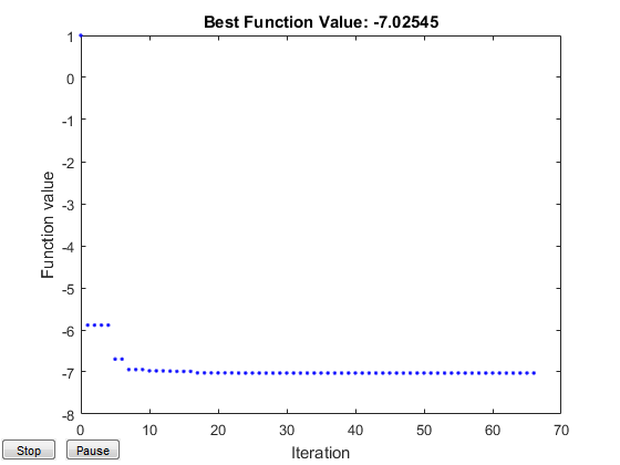
Iter     f-count          f(x)      MeshSize     Method
    0        1              1             1      
    1        4       -5.88607             2     Successful Poll
    2        8       -5.88607             1     Refine Mesh
    3       12       -5.88607           0.5     Refine Mesh
    4       16       -5.88607          0.25     Refine Mesh

(output trimmed)

   63      218       -7.02545     1.907e-06     Refine Mesh
   64      221       -7.02545     3.815e-06     Successful Poll
   65      225       -7.02545     1.907e-06     Refine Mesh
   66      229       -7.02545     9.537e-07     Refine Mesh
Optimization terminated: mesh size less than options.MeshTolerance.

x =

   -0.7037   -0.1860

Find a minimum value of a function and report both the location and value of the minimum.

Create the following two-variable objective function. On your MATLAB® path, save the following code to a file named psobj.m.

function y = psobj(x)

y = exp(-x(1)^2-x(2)^2)*(1+5*x(1) + 6*x(2) + 12*x(1)*cos(x(2)));

Set the objective function to @psobj.

fun = @psobj;

Find the unconstrained minimum of the objective, starting from the point [0,0]. Return both the location of the minimum, x, and the value of fun(x).

x0 = [0,0];
[x,fval] = patternsearch(fun,x0)
patternsearch stopped because the mesh size was less than options.MeshTolerance.

x =

   -0.7037   -0.1860


fval =

   -7.0254

To examine the patternsearch solution process, obtain all outputs.

Create the following two-variable objective function. On your MATLAB® path, save the following code to a file named psobj.m.

function y = psobj(x)

y = exp(-x(1)^2-x(2)^2)*(1+5*x(1) + 6*x(2) + 12*x(1)*cos(x(2)));

Set the objective function to @psobj.

fun = @psobj;

Find the unconstrained minimum of the objective, starting from the point [0,0]. Return the solution, x, the objective function value at the solution, fun(x), the exit flag, and the output structure.

x0 = [0,0];
[x,fval,exitflag,output] = patternsearch(fun,x0)
patternsearch stopped because the mesh size was less than options.MeshTolerance.

x =

   -0.7037   -0.1860


fval =

   -7.0254


exitflag =

     1


output = 

  struct with fields:

         function: @psobj
      problemtype: 'unconstrained'
       pollmethod: 'gpspositivebasis2n'
    maxconstraint: []
     searchmethod: []
       iterations: 66
        funccount: 229
         meshsize: 9.5367e-07
         rngstate: [1x1 struct]
          message: 'patternsearch stopped because the mesh size was less than options.MeshTolerance.'

The exitflag is 1, indicating convergence to a local minimum.

The output structure includes information such as how many iterations patternsearch took, and how many function evaluations. Compare this output structure with the results from Pattern Search with Nondefault Options. In that example, you obtain some of this information, but did not obtain, for example, the number of function evaluations.

Input Arguments

collapse all

Function to be minimized, specified as a function handle or function name. The fun function accepts a vector x and returns a real scalar f, which is the objective function evaluated at x.

You can specify fun as a function handle for a file

x = patternsearch(@myfun,x0)

Here, myfun is a MATLAB function such as

function f = myfun(x)
f = ...            % Compute function value at x

fun can also be a function handle for an anonymous function

x = patternsearch(@(x)norm(x)^2,x0,A,b);

Example: fun = @(x)sin(x(1))*cos(x(2))

Data Types: char | function_handle | string

Initial point, specified as a real vector. patternsearch uses the number of elements in x0 to determine the number of variables that fun accepts.

Example: x0 = [1,2,3,4]

Data Types: double

Linear inequality constraints, specified as a real matrix. A is an M-by-nvars matrix, where M is the number of inequalities.

A encodes the M linear inequalities

A*x <= b,

where x is the column vector of nvars variables x(:), and b is a column vector with M elements.

For example, to specify

x1 + 2x2 ≤ 10
3x1 + 4x2 ≤ 20
5x1 + 6x2 ≤ 30,

give these constraints:

A = [1,2;3,4;5,6];
b = [10;20;30];

Example: To specify that the control variables sum to 1 or less, give the constraints A = ones(1,N) and b = 1.

Data Types: double

Linear inequality constraints, specified as a real vector. b is an M-element vector related to the A matrix. If you pass b as a row vector, solvers internally convert b to the column vector b(:).

b encodes the M linear inequalities

A*x <= b,

where x is the column vector of N variables x(:), and A is a matrix of size M-by-N.

For example, to specify

x1 + 2x2 ≤ 10
3x1 + 4x2 ≤ 20
5x1 + 6x2 ≤ 30,

give these constraints:

A = [1,2;3,4;5,6];
b = [10;20;30];

Example: To specify that the control variables sum to 1 or less, give the constraints A = ones(1,N) and b = 1.

Data Types: double

Linear equality constraints, specified as a real matrix. Aeq is an Me-by-nvars matrix, where Me is the number of equalities.

Aeq encodes the Me linear equalities

Aeq*x = beq,

where x is the column vector of N variables x(:), and beq is a column vector with Me elements.

For example, to specify

x1 + 2x2 + 3x3 = 10
2x1 + 4x2 + x3 = 20,

give these constraints:

Aeq = [1,2,3;2,4,1];
beq = [10;20];

Example: To specify that the control variables sum to 1, give the constraints Aeq = ones(1,N) and beq = 1.

Data Types: double

Linear equality constraints, specified as a real vector. beq is an Me-element vector related to the Aeq matrix. If you pass beq as a row vector, solvers internally convert beq to the column vector beq(:).

beq encodes the Me linear equalities

Aeq*x = beq,

where x is the column vector of N variables x(:), and Aeq is a matrix of size Meq-by-N.

For example, to specify

x1 + 2x2 + 3x3 = 10
2x1 + 4x2 + x3 = 20,

give these constraints:

Aeq = [1,2,3;2,4,1];
beq = [10;20];

Example: To specify that the control variables sum to 1, give the constraints Aeq = ones(1,N) and beq = 1.

Data Types: double

Lower bounds, specified as a real vector or real array. If the number of elements in x0 is equal to that of lb, then lb specifies that

x(i) >= lb(i)

for all i.

If numel(lb) < numel(x0), then lb specifies that

x(i) >= lb(i)

for

1 <= i <= numel(lb)

In this case, solvers issue a warning.

Example: To specify that all control variables are positive, lb = zeros(size(x0))

Data Types: double

Upper bounds, specified as a real vector or real array. If the number of elements in x0 is equal to that of ub, then ub specifies that

x(i) <= ub(i)

for all i.

If numel(ub) < numel(x0), then ub specifies that

x(i) <= ub(i)

for

1 <= i <= numel(ub)

In this case, solvers issue a warning.

Example: To specify that all control variables are less than one, ub = ones(size(x0))

Data Types: double

Nonlinear constraints, specified as a function handle or function name. nonlcon is a function that accepts a vector or array x and returns two arrays, c(x) and ceq(x).

  • c(x) is the array of nonlinear inequality constraints at x. patternsearch attempts to satisfy

    c(x) <= 0

    for all entries of c.

  • ceq(x) is the array of nonlinear equality constraints at x. patternsearch attempts to satisfy

    ceq(x) = 0

    for all entries of ceq.

For example,

x = patternsearch(@myfun,x0,A,b,Aeq,beq,lb,ub,@mycon)

where mycon is a MATLAB function such as

function [c,ceq] = mycon(x)
c = ...     % Compute nonlinear inequalities at x.
ceq = ...   % Compute nonlinear equalities at x.
For more information, see Nonlinear Constraints.

Data Types: char | function_handle | string

Optimization options, specified as an object returned by optimoptions (recommended), or a structure.

The following table describes the optimization options. optimoptions hides the options shown in italics; see Options that optimoptions Hides. {} denotes the default value. See option details in Pattern Search Options.

Options for patternsearch

OptionDescriptionValues
Algorithm

Algorithm used by patternsearch. The Algorithm setting affects the available options. For algorithm details, see How Pattern Search Polling Works and Nonuniform Pattern Search (NUPS) Algorithm.

For examples of algorithm effects, see Explore patternsearch Algorithms and Explore patternsearch Algorithms in Optimize Live Editor Task.

{"classic"} | "nups" | "nups-gps" | "nups-mads"
Cache

With Cache set to "on", patternsearch keeps a history of the mesh points it polls. At subsequent iterations, patternsearch does not poll points close to those already polled. Use this option if patternsearch runs slowly while computing the objective function. If the objective function is stochastic, do not use this option.

Note

Cache does not work when you run the solver in parallel.

"on" | {"off"}

CacheSize

Size of the history.

Positive scalar | {1e4}

CacheTol

Largest distance from the current mesh point to any point in the history in order for patternsearch to avoid polling the current point. Use if the Cache option is set to "on".

Positive scalar | {eps}

ConstraintTolerance

Tolerance on constraints.

For an options structure, use TolCon.

Positive scalar | {1e-6}

Display

Level of display, meaning how much information patternsearch returns to the Command Line during the solution process.

"off" | "iter" | "diagnose" | {"final"}
FunctionTolerance

Tolerance on the function. Iterations stop if the change in function value is less than FunctionTolerance and the mesh size is less than StepTolerance. This option does not apply to MADS (mesh adaptive direct search) polling.

For an options structure, use TolFun.

Positive scalar | {1e-6}

InitialMeshSize

Initial mesh size for the algorithm. See How Pattern Search Polling Works.

Positive scalar | {1.0}

InitialPenalty

Initial value of the penalty parameter. See Nonlinear Constraint Solver Algorithm for Pattern Search.

Positive scalar | {10}

MaxFunctionEvaluations

Maximum number of objective function evaluations.

For an options structure, use MaxFunEvals.

Positive integer | {"2000*numberOfVariables"}, where numberOfVariables is the number of problem variables

MaxIterations

Maximum number of iterations.

For an options structure, use MaxIter.

Positive integer | {"100*numberOfVariables"}, where numberOfVariables is the number of problem variables

MaxMeshSize

Maximum mesh size used in a poll or search step. See How Pattern Search Polling Works.

Positive scalar | {Inf}

MaxTime

Total time (in seconds) allowed for optimization.

For an options structure, use TimeLimit.

Positive scalar | {Inf}

MeshContractionFactor

Mesh contraction factor for an unsuccessful iteration.

This option applies only when Algorithm is "classic".

For an options structure, use MeshContraction.

Positive scalar | {0.5}

MeshExpansionFactor

Mesh expansion factor for a successful iteration.

This option applies only when Algorithm is "classic".

For an options structure, use MeshExpansion.

Positive scalar | {2.0}

MeshRotate

Flag to rotate the pattern before declaring a point to be optimum. See Mesh Options.

This option applies only when Algorithm is "classic".

"off" | {"on"}

MeshTolerance

Tolerance on the mesh size.

For an options structure, use TolMesh.

Positive scalar | {1e-6}

OutputFcn

Function called by an optimization function at each iteration. Specify as a function handle or a cell array of function handles.

For an options structure, use OutputFcns.

Function handle or cell array of function handles | {[]}

PenaltyFactor

Penalty update parameter. See Nonlinear Constraint Solver Algorithm for Pattern Search.

Positive scalar | {100}

PlotFcn

Plots of output from the pattern search. Specify as the name of a built-in plot function, a function handle, or a cell array of names of built-in plot functions or function handles.

For an options structure, use PlotFcns.

{[]} | "psplotbestf" | "psplotfuncount" | "psplotmeshsize" | "psplotbestx" | "psplotmaxconstr" | custom plot function

PlotInterval

Number of iterations for plots. 1 means plot every iteration, 2 means plot every other iteration, and so on.

positive integer | {1}

PollMethod

Polling strategy used in the pattern search.

This option applies only when Algorithm is "classic".

Note

You cannot use MADS polling when the problem has linear equality constraints.

{"GPSPositiveBasis2N"} | "GPSPositiveBasisNp1" | "GSSPositiveBasis2N" | "GSSPositiveBasisNp1" | "MADSPositiveBasis2N" | "MADSPositiveBasisNp1"

PollOrderAlgorithm

Order of the poll directions in the pattern search.

This option applies only when Algorithm is "classic".

For an options structure, use PollingOrder.

"Random" | "Success" | {"Consecutive"}

ScaleMesh

Automatic scaling of variables.

For an options structure, use ScaleMesh = "on" or "off".

{true}| false

SearchFcn

Type of search used in the pattern search. Specify as a name or a function handle.

For an options structure, use SearchMethod.

"GPSPositiveBasis2N" | "GPSPositiveBasisNp1" | "GSSPositiveBasis2N" | "GSSPositiveBasisNp1" | "MADSPositiveBasis2N" | "MADSPositiveBasisNp1" | "searchga" | "searchlhs" | "searchneldermead" | "rbfsurrogate" | {[]} | custom search function

StepTolerance

Tolerance on the variable. Iterations stop if both the change in position and the mesh size are less than StepTolerance. This option does not apply to MADS polling.

For an options structure, use TolX.

Positive scalar | {1e-6}

TolBind

Binding tolerance. See Constraint Parameters.

Positive scalar | {1e-3}

UseCompletePoll

Flag to complete the poll around the current point. See How Pattern Search Polling Works.

This option applies only when Algorithm is "classic".

Note

For the "classic" algorithm, you must set UseCompletePoll to true for vectorized or parallel polling. Similarly, set UseCompleteSearch to true for vectorized or parallel searching.

Beginning in R2019a, when you set the UseParallel option to true, patternsearch internally overrides the UseCompletePoll setting to true so that the function polls in parallel.

For an options structure, use CompletePoll = "on" or "off".

true | {false}

UseCompleteSearch

Flag to complete the search around the current point when the search method is a poll method. See Searching and Polling.

This option applies only when Algorithm is "classic".

Note

For the "classic" algorithm, you must set UseCompleteSearch to true for vectorized or parallel searching.

For an options structure, use CompleteSearch = "on" or "off".

true | {false}

UseParallel

Flag to compute objective and nonlinear constraint functions in parallel. See Vectorized and Parallel Options and How to Use Parallel Processing in Global Optimization Toolbox.

Note

For the "classic" algorithm, you must set UseCompletePoll to true for vectorized or parallel polling. Similarly, set UseCompleteSearch to true for vectorized or parallel searching.

Beginning in R2019a, when you set the UseParallel option to true, patternsearch internally overrides the UseCompletePoll setting to true so that the function polls in parallel.

Note

Cache does not work when you run the solver in parallel.

true | {false}

UseVectorized

Specifies whether functions are vectorized. See Vectorized and Parallel Options and Vectorize the Objective and Constraint Functions.

Note

For the "classic" algorithm, you must set UseCompletePoll to true for vectorized or parallel polling. Similarly, set UseCompleteSearch to true for vectorized or parallel searching.

For an options structure, use Vectorized = "on" or "off".

true | {false}

Example: options = optimoptions("patternsearch",MaxIterations=150,MeshTolerance=1e-4)

Problem structure, specified as a structure with the following fields:

  • objective — Objective function

  • x0 — Starting point

  • Aineq — Matrix for linear inequality constraints

  • bineq — Vector for linear inequality constraints

  • Aeq — Matrix for linear equality constraints

  • beq — Vector for linear equality constraints

  • lb — Lower bound for x

  • ub — Upper bound for x

  • nonlcon — Nonlinear constraint function

  • solver'patternsearch'

  • options — Options created with optimoptions or a structure

  • rngstate — Optional field to reset the state of the random number generator

Note

All fields in problem are required except for rngstate.

Data Types: struct

Output Arguments

collapse all

Solution, returned as a real vector. The size of x is the same as the size of x0. When exitflag is positive, x is typically a local solution to the problem.

Objective function value at the solution, returned as a real number. Generally, fval = fun(x).

Reason patternsearch stopped, returned as an integer.

Exit FlagMeaning

1

Without nonlinear constraints — The magnitude of the mesh size is less than the specified tolerance, and the constraint violation is less than ConstraintTolerance.

With nonlinear constraints — The magnitude of the complementarity measure (defined after this table) is less than sqrt(ConstraintTolerance), the subproblem is solved using a mesh finer than MeshTolerance, and the constraint violation is less than ConstraintTolerance.

2

The change in x and the mesh size are both less than the specified tolerance, and the constraint violation is less than ConstraintTolerance.

3

The change in fval and the mesh size are both less than the specified tolerance, and the constraint violation is less than ConstraintTolerance.

4

The magnitude of the step is smaller than machine precision, and the constraint violation is less than ConstraintTolerance.

0

The maximum number of function evaluations or iterations is reached.

-1

Optimization terminated by an output function or plot function.

-2

No feasible point found.

In the nonlinear constraint solver, the complementarity measure is the norm of the vector whose elements are ciλi, where ci is the nonlinear inequality constraint violation, and λi is the corresponding Lagrange multiplier.

Information about the optimization process, returned as a structure with these fields:

  • function — Objective function.

  • problemtype — Problem type, one of:

    • 'unconstrained'

    • 'boundconstraints'

    • 'linearconstraints'

    • 'nonlinearconstr'

  • pollmethod — Polling technique.

  • searchmethod — Search technique used, if any.

  • iterations — Total number of iterations.

  • funccount — Total number of function evaluations.

  • meshsize — Mesh size at x.

  • maxconstraint — Maximum constraint violation, if any.

  • rngstate — State of the MATLAB random number generator, just before the algorithm started. You can use the values in rngstate to reproduce the output when you use a random search method or random poll method. See Reproduce Results, which discusses the identical technique for ga.

  • message — Reason why the algorithm terminated.

Algorithms

By default and in the absence of linear constraints, patternsearch looks for a minimum based on an adaptive mesh that is aligned with the coordinate directions. See What Is Direct Search? and How Pattern Search Polling Works.

When you set the Algorithm option to "nups" or one of its variants, patternsearch uses the algorithm described in Nonuniform Pattern Search (NUPS) Algorithm. This algorithm is different from the default algorithm in several ways; for example, it has fewer options to set.

Alternative Functionality

App

The Optimize Live Editor task provides a visual interface for patternsearch.

References

[1] Audet, Charles, and J. E. Dennis Jr. “Analysis of Generalized Pattern Searches.” SIAM Journal on Optimization. Volume 13, Number 3, 2003, pp. 889–903.

[2] Conn, A. R., N. I. M. Gould, and Ph. L. Toint. “A Globally Convergent Augmented Lagrangian Barrier Algorithm for Optimization with General Inequality Constraints and Simple Bounds.” Mathematics of Computation. Volume 66, Number 217, 1997, pp. 261–288.

[3] Abramson, Mark A. Pattern Search Filter Algorithms for Mixed Variable General Constrained Optimization Problems. Ph.D. Thesis, Department of Computational and Applied Mathematics, Rice University, August 2002.

[4] Abramson, Mark A., Charles Audet, J. E. Dennis, Jr., and Sebastien Le Digabel. “ORTHOMADS: A deterministic MADS instance with orthogonal directions.” SIAM Journal on Optimization. Volume 20, Number 2, 2009, pp. 948–966.

[5] Kolda, Tamara G., Robert Michael Lewis, and Virginia Torczon. “Optimization by direct search: new perspectives on some classical and modern methods.” SIAM Review. Volume 45, Issue 3, 2003, pp. 385–482.

[6] Kolda, Tamara G., Robert Michael Lewis, and Virginia Torczon. “A generating set direct search augmented Lagrangian algorithm for optimization with a combination of general and linear constraints.” Technical Report SAND2006-5315, Sandia National Laboratories, August 2006.

[7] Lewis, Robert Michael, Anne Shepherd, and Virginia Torczon. “Implementing generating set search methods for linearly constrained minimization.” SIAM Journal on Scientific Computing. Volume 29, Issue 6, 2007, pp. 2507–2530.

Extended Capabilities

Version History

Introduced before R2006a