Deploy Signal Classifier on NVIDIA Jetson Using Wavelet Analysis and Deep Learning

ECG Data Description and Download

The ECG data is obtained from three groups of people: persons with cardiac arrhythmia (ARR), persons with congestive heart failure (CHF), and persons with normal sinus rhythms (NSR). In total there are 162 ECG recordings from three PhysioNet databases: MIT-BIH Arrhythmia Database [2][3], MIT-BIH Normal Sinus Rhythm Database [3], and The BIDMC Congestive Heart Failure Database [1][3]. More specifically, 96 recordings from persons with arrhythmia, 30 recordings from persons with congestive heart failure, and 36 recordings from persons with normal sinus rhythms. The goal is to train a model to distinguish between ARR, CHF, and NSR.

You can obtain this data from the MathWorks GitHub repository. To download the data from the website, click Code and select Download ZIP. Save the file physionet_ECG_data-main.zip in a folder where you have write permission. The instructions for this example assume you have downloaded the file to your temporary directory, tempdir, in MATLAB®. Modify the subsequent instructions for unzipping and loading the data if you choose to download the data in a folder different from tempdir.

After downloading the data from GitHub, unzip the file in your temporary directory.

unzip(fullfile(tempdir,'physionet_ECG_data-main.zip'),tempdir)

Unzipping creates the folder physionet-ECG_data-main in your temporary directory. This folder contains the text file README.md and ECGData.zip. The ECGData.zip file contains:

ECGData.mat holds the data used in this example. The text file Modified_physionet_data.txt is required by PhysioNet's copying policy and provides the source attributions for the data as well as a description of the preprocessing steps applied to each ECG recording.

Unzip ECGData.zip in physionet-ECG_data-main. Load the data file into your MATLAB workspace.

unzip(fullfile(tempdir,'physionet_ECG_data-main','ECGData.zip'),...
    fullfile(tempdir,'physionet_ECG_data-main'))
load(fullfile(tempdir,'physionet_ECG_data-main','ECGData.mat'))

ECGData is a structure array with two fields: Data and Labels. The Data field is a 162-by-65536 matrix where each row is an ECG recording sampled at 128 hertz. Labels is a 162-by-1 cell array of diagnostic labels, one label for each row of Data. The three diagnostic categories are: 'ARR', 'CHF', and 'NSR'.

Feature Extraction

After downloading the data, you must generate scalograms of the signals. The scalograms are the "input" images to the CNN.

To store the scalograms of each category, first create an ECG data directory 'data' inside tempdir. Then create three subdirectories in 'data' named after each ECG category. The helper function helperCreateECGDirectories does this for you. helperCreateECGDirectories accepts ECGData, the name of an ECG data directory, and the name of a parent directory as input arguments. You can replace tempdir with another directory where you have write permission. You can find the source code for this helper function in the Supporting Functions section at the end of this example.

parentDir = tempdir;
dataDir = 'data';
helperCreateECGDirectories(ECGData,parentDir,dataDir)

After making the folders, create scalograms of the ECG signals as RGB images and write them to the appropriate subdirectory in dataDir. To create the scalograms, first precompute a CWT filter bank. Precomputing the filter bank is the preferred method when obtaining the CWT of many signals using the same parameters. The helper function helperCreateRGBfromTF does this. The source code for this helper function is in the Supporting Functions section at the end of this example. To be compatible with the SqueezeNet architecture, each RGB image is an array of size 227-by-227-by-3.

helperCreateRGBfromTF(ECGData,parentDir,dataDir)

Divide Data Set into Training and Validation Data

Load the scalogram images as an image datastore. The imageDatastore function automatically labels the images based on folder names and stores the data as an ImageDatastore object. An image datastore enables you to store large image data, including data that does not fit in memory, and efficiently read batches of images when training a CNN.

allImages = imageDatastore(fullfile(tempdir,dataDir),...
    'IncludeSubfolders',true,...
    'LabelSource','foldernames');

Randomly divide the images into two groups, one for training and the other for validation. Use 80% of the images for training and the remainder for validation. For purposes of reproducibility, we set the random seed to the default value.

rng default
[imgsTrain,imgsValidation] = splitEachLabel(allImages,0.8,'randomized');
disp(['Number of training images: ',num2str(numel(imgsTrain.Files))]);

Number of training images: 130

disp(['Number of validation images: ',num2str(numel(imgsValidation.Files))]);

Number of validation images: 32

SqueezeNet

SqueezeNet is a pretrained CNN that can classify images into 1000 categories. You need to retrain SqueezeNet for our ECG classification problem. Prior to retraining, you modify several network layers and set various training options. After retraining is complete, you save the CNN in a .mat file. The CUDA executable will use the .mat file.

Specify an experiment trial index and a results directory. If necessary, create the directory.

trial = 1;
ResultDir = 'results';
if ~exist(ResultDir,'dir')
    mkdir(ResultDir)
end
MatFile = fullfile(ResultDir,sprintf('SqueezeNet_Trial%d.mat',trial));

Load SqeezeNet. Extract the layer graph and inspect the last five layers.

sqz = squeezenet;
lgraph = layerGraph(sqz);
lgraph.Layers(end-4:end)

ans = 
  5×1 Layer array with layers:

     1   'conv10'                            Convolution                  1000 1×1×512 convolutions with stride [1  1] and padding [0  0  0  0]
     2   'relu_conv10'                       ReLU                         ReLU
     3   'pool10'                            2-D Global Average Pooling   2-D global average pooling
     4   'prob'                              Softmax                      softmax
     5   'ClassificationLayer_predictions'   Classification Output        crossentropyex with 'tench' and 999 other classes

To retrain SqueezeNet to classify the three classes of ECG signals, replace the 'conv10' layer with a new convolutional layer with the number of filters equal to the number of ECG classes. Replace the classification layer with a new one without class labels.

numClasses = numel(categories(imgsTrain.Labels));
new_conv10_WeightLearnRateFactor = 1;
new_conv10_BiasLearnRateFactor = 1;
newConvLayer = convolution2dLayer(1,numClasses,...
        'Name','new_conv10',...
        'WeightLearnRateFactor',new_conv10_WeightLearnRateFactor,...
        'BiasLearnRateFactor',new_conv10_BiasLearnRateFactor);
lgraph = replaceLayer(lgraph,'conv10',newConvLayer);
newClassLayer = classificationLayer('Name','new_classoutput');
lgraph = replaceLayer(lgraph,'ClassificationLayer_predictions',newClassLayer);
lgraph.Layers(end-4:end)

ans = 
  5×1 Layer array with layers:

     1   'new_conv10'        Convolution                  3 1×1 convolutions with stride [1  1] and padding [0  0  0  0]
     2   'relu_conv10'       ReLU                         ReLU
     3   'pool10'            2-D Global Average Pooling   2-D global average pooling
     4   'prob'              Softmax                      softmax
     5   'new_classoutput'   Classification Output        crossentropyex

Create a set of training options to use with SqueezeNet.

OptimSolver = 'sgdm';
MiniBatchSize = 15;
MaxEpochs = 20;
InitialLearnRate = 1e-4;
Momentum = 0.9;
ExecutionEnvironment = 'cpu';

options = trainingOptions(OptimSolver,...
    'MiniBatchSize',MiniBatchSize,...
    'MaxEpochs',MaxEpochs,...
    'InitialLearnRate',InitialLearnRate,...
    'ValidationData',imgsValidation,...
    'ValidationFrequency',10,...
    'ExecutionEnvironment',ExecutionEnvironment,...
    'Momentum',Momentum);

Save all the parameters in a structure. The trained network and structure will be later saved in a .mat file.

TrialParameter.new_conv10_WeightLearnRateFactor = new_conv10_WeightLearnRateFactor;
TrialParameter.new_conv10_BiasLearnRateFactor = new_conv10_BiasLearnRateFactor;
TrialParameter.OptimSolver = OptimSolver;
TrialParameter.MiniBatchSize = MiniBatchSize;
TrialParameter.MaxEpochs = MaxEpochs;
TrialParameter.InitialLearnRate = InitialLearnRate;
TrialParameter.Momentum = Momentum;
TrialParameter.ExecutionEnvironment = ExecutionEnvironment;

Set the random seed to the default value and train the network. Save the trained network, trial parameters, training run time, and image datastore containing the validation images. The training process usually takes 1-5 minutes on a desktop CPU. If you want to use a trained CNN from a previous trial, set trial to the index number of that trial and LoadModel to true.

LoadModel = false;
if ~LoadModel
    rng default
    tic;
    trainedModel = trainNetwork(imgsTrain,lgraph,options);
    trainingTime = toc;
    fprintf('Total training time: %.2e sec\n',trainingTime);
    save(MatFile,'TrialParameter','trainedModel','trainingTime','imgsValidation');
else
    disp('Load ML model from the file')
    load(MatFile,'trainedModel','imgsValidation');
end

Initializing input data normalization.
|======================================================================================================================|
|  Epoch  |  Iteration  |  Time Elapsed  |  Mini-batch  |  Validation  |  Mini-batch  |  Validation  |  Base Learning  |
|         |             |   (hh:mm:ss)   |   Accuracy   |   Accuracy   |     Loss     |     Loss     |      Rate       |
|======================================================================================================================|
|       1 |           1 |       00:00:03 |       26.67% |       25.00% |       4.1769 |       2.9883 |      1.0000e-04 |
|       2 |          10 |       00:00:18 |       73.33% |       59.38% |       0.9875 |       1.1554 |      1.0000e-04 |
|       3 |          20 |       00:00:35 |       60.00% |       56.25% |       0.9157 |       0.9178 |      1.0000e-04 |
|       4 |          30 |       00:00:52 |       86.67% |       68.75% |       0.6708 |       0.7883 |      1.0000e-04 |
|       5 |          40 |       00:01:10 |       66.67% |       68.75% |       0.9026 |       0.7482 |      1.0000e-04 |
|       7 |          50 |       00:01:29 |       80.00% |       78.12% |       0.5429 |       0.6788 |      1.0000e-04 |
|       8 |          60 |       00:01:48 |      100.00% |       81.25% |       0.4165 |       0.6130 |      1.0000e-04 |
|       9 |          70 |       00:02:06 |       93.33% |       84.38% |       0.3590 |       0.5480 |      1.0000e-04 |
|      10 |          80 |       00:02:24 |       73.33% |       84.38% |       0.5113 |       0.4783 |      1.0000e-04 |
|      12 |          90 |       00:02:42 |       86.67% |       84.38% |       0.4211 |       0.4065 |      1.0000e-04 |
|      13 |         100 |       00:03:00 |       93.33% |       90.62% |       0.1935 |       0.3486 |      1.0000e-04 |
|      14 |         110 |       00:03:18 |      100.00% |       90.62% |       0.1488 |       0.3119 |      1.0000e-04 |
|      15 |         120 |       00:03:36 |      100.00% |       93.75% |       0.0788 |       0.2774 |      1.0000e-04 |
|      17 |         130 |       00:03:55 |       86.67% |       93.75% |       0.2489 |       0.2822 |      1.0000e-04 |
|      18 |         140 |       00:04:13 |      100.00% |       93.75% |       0.0393 |       0.2283 |      1.0000e-04 |
|      19 |         150 |       00:04:32 |      100.00% |       93.75% |       0.0522 |       0.2364 |      1.0000e-04 |
|      20 |         160 |       00:04:50 |      100.00% |       93.75% |       0.0227 |       0.2034 |      1.0000e-04 |
|======================================================================================================================|
Training finished: Max epochs completed.

Total training time: 3.03e+02 sec

Save only the trained network in a separate .mat file. This file will be used by the CUDA executable.

ModelFile = fullfile(ResultDir,sprintf('SqueezeNet_Trial%d.mat',trial));
OutMatFile = fullfile('ecg_model.mat');

data = load(ModelFile,'trainedModel');
net = data.trainedModel;
save(OutMatFile,'net');

Use the trained network to predict the classes for the validation set.

[YPred, probs] = classify(trainedModel,imgsValidation);
accuracy = mean(YPred==imgsValidation.Labels)

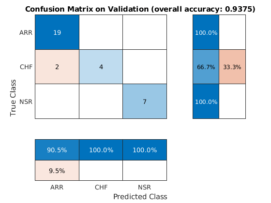
accuracy = 0.9375

Summarize the performance of the trained network on the validation set with a confusion chart. Display the precision and recall for each class by using column and row summaries. Save the figure. The table at the bottom of the confusion chart shows the precision values. The table to the right of the confusion chart shows the recall values.

figure
confusionMat = confusionmat(imgsValidation.Labels,YPred);
confusionchart(imgsValidation.Labels,YPred, ...
    'Title',sprintf('Confusion Matrix on Validation (overall accuracy: %.4f)',accuracy),...
    'ColumnSummary','column-normalized','RowSummary','row-normalized');

AccFigFile = fullfile(ResultDir,sprintf('SqueezeNet_ValidationAccuracy_Trial%d.fig',trial));
saveas(gcf,AccFigFile);

Display the size of the trained network.

info = whos('trainedModel');
ModelMemSize = info.bytes/1024;
fprintf('Trained network size: %g kB\n',ModelMemSize)

Trained network size: 2991.89 kB

Determine the average time it takes the network to classify an image.

NumTestForPredTime = 20;
TrialParameter.NumTestForPredTime = NumTestForPredTime;

fprintf('Test prediction time (number of tests: %d)... ',NumTestForPredTime)

Test prediction time (number of tests: 20)... 

imageSize = trainedModel.Layers(1).InputSize;
PredTime = zeros(NumTestForPredTime,1);
for i = 1:NumTestForPredTime
    x = randn(imageSize);
    tic;
    [YPred, probs] = classify(trainedModel,x,'ExecutionEnvironment',ExecutionEnvironment);
    PredTime(i) = toc;
end
AvgPredTimePerImage = mean(PredTime);
fprintf('Average prediction time (execution environment: %s): %.2e sec \n',...
    ExecutionEnvironment,AvgPredTimePerImage);

Average prediction time (execution environment: cpu): 1.67e-01 sec 

Save the results.

if ~LoadModel
    save(MatFile,'accuracy','confusionMat','PredTime','ModelMemSize', ...
        'AvgPredTimePerImage','-append')
end

GPU Code Generation — Define Functions

The scalogram of a signal is the input "image" to a deep CNN. Create a function, cwt_ecg_jetson_ex, that computes the scalogram of an input signal and returns an image at the user-specified dimensions. The image uses the jet(128) colormap. The %#codegen directive in the function indicates that the function is intended for code generation. When using the coder.gpu.kernelfun pragma, code generation attempts to map the computations in the cwt_ecg_jetson_ex function to the GPU.

type cwt_ecg_jetson_ex.m

function im = cwt_ecg_jetson_ex(TimeSeriesSignal, ImgSize) %#codegen
% This function is only intended to support wavelet deep learning examples.
% It may change or be removed in a future release.

coder.gpu.kernelfun();

%% Create Scalogram
cfs = cwt(TimeSeriesSignal, 'morse', 1, 'VoicesPerOctave', 12);
cfs = abs(cfs);

%% Image generation
cmapj128 = coder.load('cmapj128');
imx = ind2rgb_custom_ecg_jetson_ex(round(255*rescale(cfs))+1,cmapj128.cmapj128);

% resize to proper size and convert to uint8 data type
im = im2uint8(imresize(imx, ImgSize)); 

end

Create the entry-point function, model_predict_ecg.m, for code generation. The function takes an ECG signal as input and calls the cwt_ecg_jetson_ex function to create an image of the scalogram. The model_predict_ecg function uses the network contained in the ecg_model.mat file to classify the ECG signal.

type model_predict_ecg.m

function PredClassProb = model_predict_ecg(TimeSeriesSignal) %#codegen
% This function is only intended to support wavelet deep learning examples.
% It may change or be removed in a future release.
    coder.gpu.kernelfun();
    
    % parameters
    ModFile = 'ecg_model.mat'; % file that saves neural network model
    ImgSize = [227 227]; % input image size for the ML model
    
    % sanity check signal is a row vector of correct length
    assert(isequal(size(TimeSeriesSignal), [1 65536])) 
    %% cwt transformation for the signal
    im = cwt_ecg_jetson_ex(TimeSeriesSignal, ImgSize);
    
    %% model prediction
    persistent model;
    if isempty(model)
        model = coder.loadDeepLearningNetwork(ModFile, 'mynet');
    end

    PredClassProb = predict(model, im);
    
end

To generate a CUDA executable that can be deployed to an NVIDIA target, create a custom main file (main_ecg_jetson_ex.cu) and a header file (main_ecg_jetson_ex.h). You can generate an example main file and use that as a template to rewrite new main and header files. For more information, see the GenerateExampleMain property of coder.CodeConfig. The main file calls the code generated for the MATLAB entry-point function. The main file first reads the ECG signal from a text file, passes the data to the entry-point function, and writes the prediction results to a text file (predClassProb.txt). To maximize computation efficiency on the GPU, the executable processes single-precision data.

type main_ecg_jetson_ex.cu

//
// File: main_ecg_jetson_ex.cu
//
// This file is only intended to support wavelet deep learning examples.
// It may change or be removed in a future release.
        
//***********************************************************************
// Include Files
#include "rt_nonfinite.h"
#include "model_predict_ecg.h"
#include "main_ecg_jetson_ex.h"
#include "model_predict_ecg_terminate.h"
#include "model_predict_ecg_initialize.h"
#include <stdio.h>
#include <stdlib.h>
#include <time.h>

// Function Definitions

/* Read data from a file*/
int readData_real32_T(const char * const file_in, real32_T data[65536])
{
  FILE* fp1 = fopen(file_in, "r");
  if (fp1 == 0)
  {
    printf("ERROR: Unable to read data from %s\n", file_in);
    exit(0);
  }
  for(int i=0; i<65536; i++)
  {
      fscanf(fp1, "%f", &data[i]);
  }
  fclose(fp1);
  return 0;
}

/* Write data to a file*/
int writeData_real32_T(const char * const file_out, real32_T data[3])
{
  FILE* fp1 = fopen(file_out, "w");
  if (fp1 == 0) 
  {
    printf("ERROR: Unable to write data to %s\n", file_out);
    exit(0);
  }
  for(int i=0; i<3; i++)
  {
    fprintf(fp1, "%f\n", data[i]);
  }
  fclose(fp1);
  return 0;
}

// model predict function
static void main_model_predict_ecg(const char * const file_in, const char * const file_out)
{
  real32_T PredClassProb[3];
  //  real_T b[65536];
  real32_T b[65536];

  // readData_real_T(file_in, b);
  readData_real32_T(file_in, b);
       
  model_predict_ecg(b, PredClassProb);

  writeData_real32_T(file_out, PredClassProb);

}

// main function
int32_T main(int32_T argc, const char * const argv[])
{
  const char * const file_out = "predClassProb.txt";
  // Initialize the application.
  model_predict_ecg_initialize();
  
  // Run prediction function
  main_model_predict_ecg(argv[1], file_out); // argv[1] = file_in

  // Terminate the application.
  model_predict_ecg_terminate();
  return 0;
}

type main_ecg_jetson_ex.h

//
// File: main_ecg_jetson_ex.h
//
// This file is only intended to support wavelet deep learning examples.
// It may change or be removed in a future release.

//
//***********************************************************************
#ifndef MAIN_H
#define MAIN_H

// Include Files
#include <stddef.h>
#include <stdlib.h>
#include "rtwtypes.h"
#include "model_predict_ecg_types.h"

// Function Declarations
extern int32_T main(int32_T argc, const char * const argv[]);

#endif

//
// File trailer for main_ecg_jetson_ex.h
//
// [EOF]
//

GPU Code Generation — Specify Target

To create an executable that can be deployed to the target device, set CodeGenMode equal to 1. If you want to create an executable that runs locally and connects remotely to the target device, set CodeGenMode equal to 2.

The main function reads data from the text file specified by signalFile and writes the classification results to resultFile. Set ExampleIndex to choose a representative ECG signal. You will use this signal to test the executable against the classify function. Jetson_BuildDir specifies the directory for performing the remote build process on the target. If the specified build directory does not exist on the target, then the software creates a directory with the given name.

CodeGenMode = 1;
signalFile = 'signalData.txt';
resultFile = 'predClassProb.txt'; % consistent with "main_ecg_jetson_ex.cu"
Jetson_BuildDir = '~/projectECG';
ExampleIndex = 1; % 1,4: type ARR; 2,5: type CHF; 3,6: type NSR

Function_to_Gen = 'model_predict_ecg';
ModFile = 'ecg_model.mat'; % file that saves neural network model; consistent with "main_ecg_jetson_ex.cu"
ImgSize = [227 227]; % input image size for the ML model

switch ExampleIndex
    case 1 % ARR 7
        SampleSignalIdx = 7;
    case 2 % CHF 97
        SampleSignalIdx = 97;
    case 3 % NSR 132
        SampleSignalIdx = 132;
    case 4 % ARR 31
        SampleSignalIdx = 31;
    case 5 % CHF 101
        SampleSignalIdx = 101;
    case 6 % NSR 131
        SampleSignalIdx = 131;
end
signal_data = single(ECGData.Data(SampleSignalIdx,:));
ECGtype = ECGData.Labels{SampleSignalIdx};

GPU Code Generation — Connect to Hardware

To communicate with the NVIDIA hardware, you create a live hardware connection object using the jetson function. You must know the host name or IP address, user name, and password of the target board to create a live hardware connection object.

Create a live hardware connection object for the Jetson hardware. In the following code, replace:

During the creation of the object, the software performs hardware and software checks, IO server installation, and gathers information on the peripherals connected to the target. This information is displayed in the command window.

hwobj = jetson("NameOfJetsonDevice","Username","password");

Checking for CUDA availability on the Target...
Checking for 'nvcc' in the target system path...
Checking for cuDNN library availability on the Target...
Checking for TensorRT library availability on the Target...
Checking for prerequisite libraries is complete.
Gathering hardware details...
Checking for third-party library availability on the Target...
Gathering hardware details is complete.
 Board name              : NVIDIA Jetson Nano
 CUDA Version            : 10.0
 cuDNN Version           : 7.3
 TensorRT Version        : 5.0
 GStreamer Version       : 1.14.5
 V4L2 Version            : 1.14.2-1
 SDL Version             : 1.2
 OpenCV Version          : 3.3.1
 Available Webcams       :  
 Available GPUs          : NVIDIA Tegra X1
 Available Digital Pins  : 7  11  12  13  15  16  18  19  21  22  23  24  26  29  31  32  33  35  36  37  38  40

Use the coder.checkGpuInstall function and verify that the compilers and libraries needed for running this example are set up correctly on the hardware.

envCfg = coder.gpuEnvConfig('jetson');
envCfg.DeepLibTarget = 'cudnn';
envCfg.DeepCodegen = 1;
envCfg.HardwareObject = hwobj;
envCfg.Quiet = 1;
coder.checkGpuInstall(envCfg)

ans = struct with fields:
                 gpu: 1
                cuda: 1
               cudnn: 1
            tensorrt: 0
        basiccodegen: 0
       basiccodeexec: 0
         deepcodegen: 1
        deepcodeexec: 0
    tensorrtdatatype: 0
           profiling: 0

GPU Code Generation — Compile

Create a GPU code configuration object necessary for compilation. Use the coder.hardware function to create a configuration object for the Jetson platform and assign it to the Hardware property of the code configuration object cfg. Use 'NVIDIA Jetson' for the Jetson TX1 or TX2 boards. The custom main file is a wrapper that calls the entry-point function in the generated code. The custom file is required for a deployed executable.

Use the coder.DeepLearningConfig function to create a CuDNN deep learning configuration object and assign it to the DeepLearningConfig property of the GPU code configuration object. The code generator takes advantage of NVIDIA® CUDA® deep neural network library (cuDNN) for NVIDIA GPUs. cuDNN is a GPU-accelerated library of primitives for deep neural networks.

if CodeGenMode == 1
    cfg = coder.gpuConfig('exe');
    cfg.Hardware = coder.hardware('NVIDIA Jetson');
    cfg.Hardware.BuildDir = Jetson_BuildDir;
    cfg.DeepLearningConfig = coder.DeepLearningConfig('cudnn');
    cfg.CustomSource = fullfile('main_ecg_jetson_ex.cu');
elseif CodeGenMode == 2
    cfg = coder.gpuConfig('lib');
    cfg.VerificationMode = 'PIL';
    cfg.Hardware = coder.hardware('NVIDIA Jetson');
    cfg.Hardware.BuildDir = Jetson_BuildDir;
    cfg.DeepLearningConfig = coder.DeepLearningConfig('cudnn');
end

To generate CUDA code, use the codegen function and pass the GPU code configuration along with the size and type of the input for the model_predict_ecg entry-point function. After code generation on the host is complete, the generated files are copied over and built on the target.

codegen('-config ',cfg,Function_to_Gen,'-args',{signal_data},'-report');

Code generation successful: View report

GPU Code Generation — Execute

If you compiled an executable to be deployed to the target, write the example ECG signal to a text file. Use the putFile() function of the hardware object to place the text file on the target. The workspaceDir property contains the path to the codegen folder on the target.

if CodeGenMode == 1
    fid = fopen(signalFile,'w');
    for i = 1:length(signal_data)
        fprintf(fid,'%f\n',signal_data(i));
    end
    fclose(fid);
    hwobj.putFile(signalFile,hwobj.workspaceDir);
end

Run the executable.

When running the deployed executable, delete the previous result file if it exists. Use the runApplication() function to launch the executable on the target hardware, and then the getFile() function to retrieve the results. Because the results may not exist immediately after the runApplication() function call returns, and to allow for communication delays, set a maximum time for fetching the results to 90 seconds. Use the evalc function to suppress the command-line output.

if CodeGenMode == 1 % run deployed executable
    maxFetchTime = 90;
    resultFile_hw = fullfile(hwobj.workspaceDir,resultFile);
    if ispc
        resultFile_hw = strrep(resultFile_hw,'\','/');
    end
    
    ta = tic;
    
    hwobj.deleteFile(resultFile_hw)
    evalc('hwobj.runApplication(Function_to_Gen,signalFile)');
    
    tf = tic;
    success = false;
    while toc(tf) < maxFetchTime
        try
            evalc('hwobj.getFile(resultFile_hw)');
            success = true;
        catch ME
        end
        if success
            break
        end
    end
    fprintf('Fetch time = %.3e sec\n',toc(tf));
    assert(success,'Unable to fetch the prediction')
    PredClassProb = readmatrix(resultFile);
    PredTime = toc(ta);
elseif CodeGenMode == 2 % run PIL executable
    ta = tic;
    eval(sprintf('PredClassProb = %s_pil(signal_data);',Function_to_Gen));
    PredTime = toc(ta);
    eval(sprintf('clear %s_pil;',Function_to_Gen)); % terminate PIL execution
end

Fetch time = 1.658e+01 sec

Use the classify function to predict the class labels for the example signal.

ModData = load(ModFile,'net');
im = cwt_ecg_jetson_ex(signal_data,ImgSize);
[ModPred, ModPredProb] = classify(ModData.net,im);
PredCat = categories(ModPred)';

Compare the results.

PredTableJetson = array2table(PredClassProb(:)','VariableNames',matlab.lang.makeValidName(PredCat));
fprintf('tPred = %.3e sec\nExample ECG Type: %s\n',PredTime,ECGtype)

tPred = 2.044e+01 sec
Example ECG Type: ARR

disp(PredTableJetson)

      ARR        CHF         NSR   
    _______    ________    ________

    0.99858    0.001252    0.000166

PredTableMATLAB = array2table(ModPredProb(:)','VariableNames',matlab.lang.makeValidName(PredCat));
disp(PredTableMATLAB)

      ARR         CHF          NSR    
    _______    _________    __________

    0.99858    0.0012516    0.00016613

Close the hardware connection.

clear hwobj

Summary

This example shows how to create and deploy a CUDA executable that uses a CNN to classify ECG signals. You also have the option to create an executable the runs locally and connects to the remote target. A complete workflow is presented in this example. After the data is downloaded, the CWT is used to extract features from the ECG signals. Then SqueezeNet is retrained to classify the signals based on their scalograms. Two user-defined functions are created and compiled on the target NVIDIA device. Results of the executable are compared with MATLAB.

References

Supporting Functions

helperCreateECGDirectories

function helperCreateECGDirectories(ECGData,parentFolder,dataFolder)
% This function is only intended to support wavelet deep learning examples.
% It may change or be removed in a future release.

rootFolder = parentFolder;
localFolder = dataFolder;
mkdir(fullfile(rootFolder,localFolder))

folderLabels = unique(ECGData.Labels);
for i = 1:numel(folderLabels)
    mkdir(fullfile(rootFolder,localFolder,char(folderLabels(i))));
end
end

helperPlotReps

function helperPlotReps(ECGData)
% This function is only intended to support wavelet deep learning examples.
% It may change or be removed in a future release.

folderLabels = unique(ECGData.Labels);

for k=1:3
    ecgType = folderLabels{k};
    ind = find(ismember(ECGData.Labels,ecgType));
    subplot(3,1,k)
    plot(ECGData.Data(ind(1),1:1000));
    grid on
    title(ecgType)
end
end

helperCreateRGBfromTF

function helperCreateRGBfromTF(ECGData,parentFolder, childFolder)
% This function is only intended to support wavelet deep learning examples.
% It may change or be removed in a future release.

imageRoot = fullfile(parentFolder,childFolder);

data = ECGData.Data;
labels = ECGData.Labels;

[~,signalLength] = size(data);

fb = cwtfilterbank('SignalLength',signalLength,'VoicesPerOctave',12);
r = size(data,1);

for ii = 1:r
    cfs = abs(fb.wt(data(ii,:)));
    im = ind2rgb(im2uint8(rescale(cfs)),jet(128));
    
    imgLoc = fullfile(imageRoot,char(labels(ii)));
    imFileName = strcat(char(labels(ii)),'_',num2str(ii),'.jpg');
    imwrite(imresize(im,[227 227]),fullfile(imgLoc,imFileName));
end
end

References

Baim, D. S., W. S. Colucci, E. S. Monrad, H. S. Smith, R. F. Wright, A. Lanoue, D. F. Gauthier, B. J. Ransil, W. Grossman, and E. Braunwald. "Survival of patients with severe congestive heart failure treated with oral milrinone." Journal of the American College of Cardiology. Vol. 7, Number 3, 1986, pp. 661–670.
Goldberger A. L., L. A. N. Amaral, L. Glass, J. M. Hausdorff, P. Ch. Ivanov, R. G. Mark, J. E. Mietus, G. B. Moody, C.-K. Peng, and H. E. Stanley. "PhysioBank, PhysioToolkit,and PhysioNet: Components of a New Research Resource for Complex Physiologic Signals." Circulation. Vol. 101, Number 23: e215–e220. [Circulation Electronic Pages;
http://circ.ahajournals.org/content/101/23/e215.full]; 2000 (June 13). doi: 10.1161/01.CIR.101.23.e215.Moody, G. B., and R. G. Mark. "The impact of the MIT-BIH Arrhythmia Database." IEEE Engineering in Medicine and Biology Magazine. Vol. 20. Number 3, May-June 2001, pp. 45–50. (PMID: 11446209)