Estimate ARMA Model Using Time Series Modeler app

The Time Series Modeler app trains models for time series modeling. This topic explains how to train an autoregressive moving average (ARMA) model using the Time Series Modeler app. This app requires Deep Learning Toolbox™.

Using this app, you can:

Import and visualize time series data.
Specify data preprocessing options such as splitting the data into training and validation sets.
Select the ARMA model type from a list of predefined models. You can identify ARMA models by using linear identification algorithms in the System Identification Toolbox™ software.
Configure the ARMA model by specifying model structure and training options.
Visualize training metrics and select a trained model from a list of candidate models.
Compare the predictions of your trained model to the measured training and validation data sets.
Export the trained model and generate MATLAB^® code to help you predict on new data.

For more information on the app, see Time Series Modeler (Deep Learning Toolbox).

Open App and Import Data

To open the Time Series Modeler app, at the MATLAB command prompt, enter timeSeriesModeler. You can also open the app by selecting Time Series Modeler from the MATLAB Apps gallery.

To import data from the MATLAB workspace into the app, on the toolstrip, click New. The Import Data dialog box opens.

Data

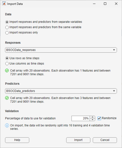
In the Data section of the Import Data dialog box, choose one of these options. Each choice gives you a different set of options to configure.

Import responses and predictors from separate variables — This option allows you to choose different variables for responses (outputs) and predictors (inputs).
Import responses and predictors from the same variable — This option allows you to choose a variable and set each of its features as either a predictor or a response.
Import responses only — This option allows you to train a time series model, which uses only responses and no inputs. For more information, see Time Series Analysis.

Responses

The Responses section of the Import Data dialog box appears when you choose Import responses and predictors from separate variables or Import responses only in the Data section.

In the Responses list, select a variable to use to train your model, specified as a numeric array, cell array, table, or timetable object. In system identification, responses are commonly called as Outputs. This is the time series you want to model and predict response. For timetable data, the data must be sampled at regular intervals. For other input types, the app assumes that the data is sampled at regular intervals.
Specify the format of the time series data:
- If your data is in the (time, channel) format, select Use rows as time steps. This option is selected by default.
- If your data is in the (channel, time) format, select Use columns as time steps.

For each option, the app displays information about your data, such as the number of time series (number of experiments), number of features, and length of the time steps. Use this information to check that you have specified the correct time dimension.

Data Set Variable

The Data Set Variable section appears when you choose Import responses and predictors from the same variable in the Data section.

In the Data Set Variable list, select a variable to use to train your model, specified as a numeric array, cell array, table, or timetable object. For timetable data, the data must be sampled at regular intervals. For other input types, the app assumes that the data is sampled at regular intervals.
Specify the format of the time series data:
- If your data is in the (time, channel) format, select Use rows as time steps. This option is selected by default.
- If your data is in the (channel, time) format, select Use columns as time steps.

Predictors

The Predictors section appears when you choose Import responses and predictors from separate variables or Import responses and predictors from the same variable in the Data section.

If you choose Import responses and predictors from separate variables, first, select a variable under Responses. In the Predictors list, select additional variables that are related to but are not part of, the time series you want to model, specified as a numeric array, cell array, table, or timetable object. In system identification, predictors are commonly called as Inputs. These are external time series that influence the responses. The data type of the predictors must match that of the responses. The app assumes that the input data is sampled at regular intervals.
If you choose Import responses and predictors from the same variable, first, select a variable under Data Set Variable. In the Predictors table, for each feature, select Predictor to set the feature as a predictor or select Response to set the feature as a response. If your data set variable has only one feature, then you can set that feature only as a response.

Validation

In the Validation section, specify the percentage of data to use for validation. Monitoring the performance of the model on the validation data is important for detecting overfitting. Suppose that you specify Validation as a value val. The validation split depends on how many time series are in the imported data.

If you have a single time series, then the validation data is the last val% of the time steps. For example, if you have a single time series with 100 time steps and a validation split of 30%, then the app uses the first 70 time steps for training and the last 30 time steps for validation.
If you have multiple time series, then the validation data is val% of the time series. For example, if you have 100 time series and a validation split of 30%, then the app uses 70 time series for training and 30 time series for validation.

If you have multiple experiments, the Randomize check box appears. Select Randomize to randomly assign the specified proportion of experiments to the validation data set. Randomizing the validation data can improve the accuracy of networks that were trained on nonrandomly ordered data.

Import Data dialog box

Preview Imported Data

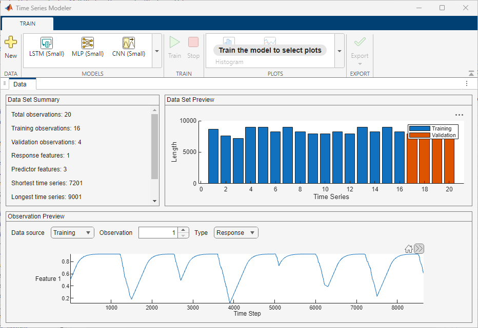
The app displays the data you import in the Data tab. In this tab:

A summary of the imported data appears in the Data Set Summary section.
You can preview individual observations in the Observation Preview section.
If the imported data includes multiple experiments, you can also view a plot of the experiments and their corresponding time steps in the Data Set Preview section.

Data tab in the app

Configure ARMA Model Structure and Training Options

ARMA Models Background

The general form of an autoregressive moving average with exogenous input (ARMAX) model is $A (q) y (t) = B (q) u (t) + C (q) e (t)$ , where

y(t) — Output at time t
u(t) — Input on which the current output depends
e(t) — White-noise disturbance
q^-1 — Delay operator, where q^-1y(t) is equivalent to y(t-1)
A(q) — $1 + a_{1} q^{- 1} + \dots + a_{n a} q^{- n a}$ , where na is the number of poles in the model
B(q) — $q^{- n k} (b_{0} + \dots + b_{n b - 1} q^{- n b + 1})$ , where nb is the number of zeros in the model plus one and nk is the number of input samples that occur before the input affects the output (delay)
C(q) — $1 + c_{1} q^{- 1} + \dots + c_{n c} q^{- n c}$ , where nc is the number of C coefficients

When you integrate the noise, the ARMAX model becomes the autoregressive moving integrated moving average with exogenous input (ARIMAX) model. The general form of an ARIMAX model is: $A (q) y (t) = B (q) u (t) + \frac{C (q)}{1 - q^{- 1}} e (t)$ .

The ARMA model is a special case of an ARMAX model with no inputs, leading to the equation: $A (q) y (t) = C (q) e (t)$ .

Model Structure Configuration

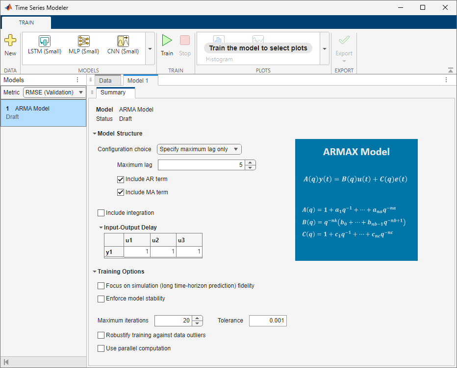
To configure the ARMA model structure you want to train, in the app, select ARMA Model from the Models gallery. The Model tab opens in the app along with its Summary tab.

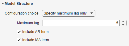
In the Summary tab, specify the structure of the model by using these options under Model Structure:

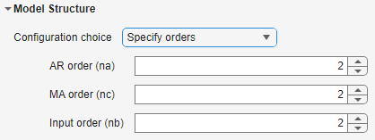
Configuration choice — Select Configuration choice as either Specify maximum lag only or Specify orders. Each choice gives you a different set of options to configure. If you select Specify maximum lag only, the app searches for the most optimal orders of the ARMAX polynomial.

Configuration choice	Description	Configuration options	Description
`Specify maximum lag only`	Specify maximum lag in the model.	Maximum lag	Specify the maximum number of past lags in the imported response and predictor values that are used to predict the current model output, as a positive scalar. The maximum lag you specify must be greater than the values in the Input-Output Delay matrix (whose default values are one).
		Include AR term	Select this option to include the autoregressive term, A(q), in the model structure.
		Include MA term	Select this option to include the moving average term, C(q), in the model structure.
`Specify orders`	Specify orders of the model.	AR order (na)	Specify the number of poles in the model, as a nonnegative integer. The value you specify is the order of the polynomial A(q).
		MA order (nc)	Specify the order of the polynomial C(q), as a nonnegative integer.
		Input order (nb)	Specify the number of zeros in the model plus one, as a nonnegative integer. The value you specify is the length of the polynomial B(q).

Include integration — Select this option to include the integrator in the model structure.
Input-Output Delay — This option appears only when you import both responses and predictors. Use this option to specify the input-output delay, also called the transport delay, as an N_y-by-N_u matrix of nonnegative integers. Here, N_y is the number of outputs and N_u is the number of inputs. If you select the Configuration choice as Specify maximum lag only, then the values you specify in the Input-Output Delay matrix must be less than the Maximum lag value.

The type of model you create depends on the data you import and the model structure you specify. This table shows how to create each type of model.

Model Type	Equation	Creation
Autoregressive (AR) model	$A (q) y (t) = e (t)$	Import data containing only responses and no predictors. Include the AR term. That is, select the Include AR term option or specify AR order (na) as a positive integer. Exclude the MA term. That is, clear the Include MA term option or specify MA order (nc) as zero.
Autoregressive Integrated (ARI) model	$A (q) y (t) = \frac{1}{1 - q^{- 1}} e (t)$	Follow the steps to create an AR model. Select the Include integration option.
Autoregressive Moving Average (ARMA) model	$A (q) y (t) = C (q) e (t)$	Import data containing only responses and no predictors. Select the Include AR term option or specify AR order (na) as a positive integer. Select the Include MA term option or specify MA order (nc) as a positive integer.
Autoregressive Integrated Moving Average (ARIMA) model	$A (q) y (t) = \frac{C (q)}{1 - q^{- 1}} e (t)$	Follow the steps to create an ARMA model. Select the Include integration option.
Moving Average (MA) model	$y (t) = C (q) e (t)$	Import data containing only responses and no predictors. Clear the Include AR term option or specify AR order (na) as zero. Select the Include MA term option or specify MA order (nc) as a positive integer.
Integrated Moving Average (IMA) model	$y (t) = \frac{C (q)}{1 - q^{- 1}} e (t)$	Follow the steps to create an MA model. Select the Include integration option.
Autoregressive with Exogenous Input (ARX) model	$A (q) y (t) = B (q) u (t) + e (t)$	Import data containing both responses and predictors. Select the Include AR term option or specify AR order (na) as a positive integer. Clear the Include MA term option or specify MA order (nc) as zero.
Autoregressive Integrated with Exogenous Input (ARIX) model	$A (q) y (t) = B (q) u (t) + \frac{1}{1 - q^{- 1}} e (t)$	Follow the steps to create an ARX model. Select the Include integration option.
Autoregressive Moving Average with Exogenous Input (ARMAX) model	$A (q) y (t) = B (q) u (t) + C (q) e (t)$	Import data containing both responses and predictors. Select the Include AR term option or specify AR order (na) as a positive integer. Select the Include MA term option or specify MA order (nc) as a positive integer.
Autoregressive Integrated Moving Average with Exogenous Input (ARIMAX) model	$A (q) y (t) = B (q) u (t) + \frac{C (q)}{1 - q^{- 1}} e (t)$	Follow the steps to create an ARMAX model. Select the Include integration option.
Moving Average with Exogenous Input (MAX) model	$y (t) = B (q) u (t) + C (q) e (t)$	Import data containing both responses and predictors. Clear the Include AR term option or specify AR order (na) as zero. Select the Include MA term option or specify MA order (nc) as a positive integer.
Integrated Moving Average with Exogenous Input (IMAX) model	$y (t) = B (q) u (t) + \frac{C (q)}{1 - q^{- 1}} e (t)$	Follow the steps to create an MAX model. Select the Include integration option.
Finite Impulse Response (FIR) model	$y (t) = B (q) u (t) + e (t)$	Import data containing both responses and predictors. Clear the Include AR term option or specify AR order (na) as zero. Clear the Include MA term option or specify MA order (nc) as zero.
Integrated Finite Impulse Response (IFIR) model	$y (t) = B (q) u (t) + \frac{1}{1 - q^{- 1}} e (t)$	Follow the steps to create an FIR model. Select the Include integration option.

Training Options Configuration

To control how the app trains the model, specify these options under Training Options in the Summary tab:

Focus on simulation (long time-horizon prediction) fidelity — Select this option to minimize the simulation error between measured and simulated outputs during estimation. The estimation focuses on making a good fit for simulation of model response with the current inputs. This option is available only when you import both responses and predictors.
Enforce model stability — Select this option to enforce stability of the estimated model.
Maximum iterations — Specify the maximum number of iterations during loss-function minimization, as a nonnegative integer. The iterations stop when MaxIterations is reached or another stopping criterion is satisfied, such as Tolerance. If you specify MaxIterations as 0, the training returns the result of the start-up procedure.
Tolerance — Specify the minimum percentage difference between the value of the loss function at each iteration and its expected value after the next iteration, as a positive scalar. When the percentage of expected improvement is less than Tolerance, the iterations stop. The estimate of the expected loss-function improvement at the next iteration is based on the Gauss-Newton vector computed for the current parameter value.
Robustify training against data outliers — Select this option to strengthen training against data outliers.
Use parallel computation — Select this option to enable parallel computing for model training. Use parallel computing to simultaneously train multiple candidate models based on the model structure you specify.

ARMA Model configuration options in the app

Train ARMA Model

To train the configured ARMA model, on the toolstrip, click Train. The Model Selector tab opens next to the Summary tab. The Training Information section appears with the statement: Trying various model structures and fitting algorithms….

During model training, the app searches for optimal model orders using arxstruc and n4sid. It searches for all possible combinations of the orders of the AR (na), MA (nc), and the input (nb) terms. If the number of combinations is more than 1e4, the app searches for only a subset of these possible combinations by refining the search in the neighborhood of the optimal results returned by the search.

The app tries a variety of training methods using both the original time-series data and its frequency-domain version. You obtain the frequency-domain version of the data by computing the fast Fourier transform of the data (for more information, see fft). The training methods include arx, armax, ssest, and tfest. During these trials, if the training data has more than 1e4 samples, the app reduces the training time by using only a portion of the data. If you import data with one response and no inputs (scalar time series data), then the app uses the ar function and trains the model using the entire data set.

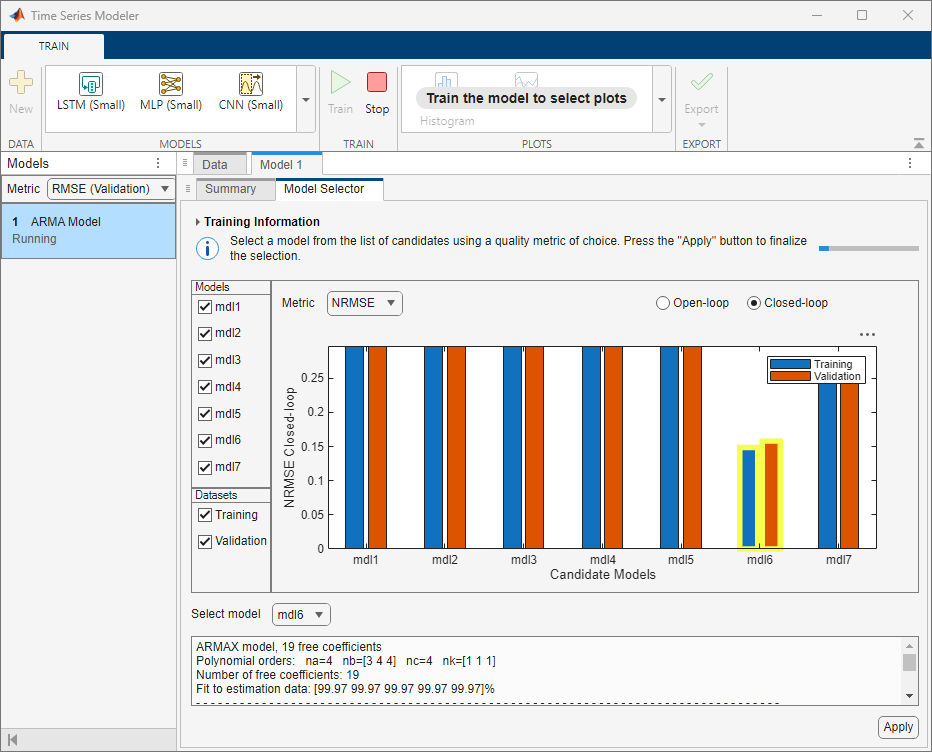
Model Selection

After model training, the app produces between one and seven candidate models. A plot displaying the candidate models and their respective metric values appears on the Model Selector tab. At the top of the plot, in the Metric menu, choose the quality metric that you want the plot to display. The available metrics are:

Quality Metric	Description
`RMSE`	Root Mean Squared Error, defined as $R M S E = \sqrt{\frac{1}{N} \sum_{t = 1}^{N} e^{T} (t) e (t)},$ where: e(t) is the signal whose norm is minimized for estimation. e(t)=y_measured(t)-y_model(t), where y_measured(t) is the measured output data and y_model(t) is the simulated or predicted response of the model. N is the number of data samples in the estimation dataset.
`NRMSE`	Normalized Root Mean Squared Error, defined as $N R M S E = \frac{\| \| e (t) \| \|}{\| \| y_{m e a s u r e d} (t) - \bar{y_{m e a s u r e d} (t)} \| \|},$ where: e(t) is the signal whose norm is minimized for estimation. y_measured(t) is the measured output data. $\bar{y_{m e a s u r e d} (t)}$ is the channel-wise mean of the measured output data. \|\|.\|\| indicates the 2-norm of the vectors.
`MAE`	Mean Absolute Error, defined as $M A E = \frac{1}{N} \sum_{t = 1}^{N} \| e (t) \|,$ where: e(t) is the signal whose norm is minimized for estimation. N is the number of data samples in the estimation dataset.
`AIC`	A raw measure of Akaike's Information Criterion, defined as $A I C = N * l o g (d e t (\frac{1}{N} E^{T} E)) + 2 * n_{p} + N (n_{y} * \log (2 π) + 1)$ where: N is the number of data samples in the estimation dataset. E is the N-by-n_y matrix of prediction errors, where n_y is the number of output channels. n_p is the number of free parameters in the model. n_p includes the number of estimated initial states.
`BIC`	Bayesian Information Criterion, defined as $B I C = N * l o g (d e t (\frac{1}{N} E^{T} E)) + N * (n_{y} * \log (2 π) + 1) + n_{p} * log (N)$ where: N is the number of data samples in the estimation dataset. E is the N-by-n_y matrix of prediction errors, where n_y is the number of output channels. n_p is the number of free parameters in the model. n_p includes the number of estimated initial states.

To the left of the plot, in the Models section, you can choose which models to display. In the Datasets section, you can choose to display the Training dataset, Validation dataset, or both.

If you choose RMSE, NRMSE, or MAE as the metric to display, then you can select Open-loop or Closed-loop at the top right of the plot to display the respective plots.

Metric Generation Setting	Description
Open-loop	Selecting the metric setting as Open-loop is equivalent to specifying the prediction horizon input argument for the `predict` and `compare` commands as `1`.
Closed-loop	Selecting the metric setting as Closed-loop is equivalent to specifying the prediction horizon input argument for the `predict` and `compare` commands as `Inf`, that is, performing a simulation of the model.

The plot automatically highlights the model with the lowest NRMSE value on training data in the closed-loop metric setting. You can also see that the app selects this model in the Select model list and displays its information in the text box below the plot. You can select a different model by clicking the model in the plot or selecting it in the Select model list.

The qualities of the candidate models change based on the metric type and metric setting you choose. A candidate model with a lower value for your chosen metric is better. When selecting a model, you can also weigh the value of the chosen metric against the complexity of the model. The number of free coefficients mentioned in the text box below the plot indicates the model complexity.

If the app produces more than one candidate model, then select a model and click Apply to complete the training process with that model. If the app produces only one candidate model, then it automatically selects that model and completes the training process. In this case, the app does not wait for you to click Apply. If the training data contains more than 1e4 samples, then the app refines the parameters of the selected model using the entire training data before returning the result.

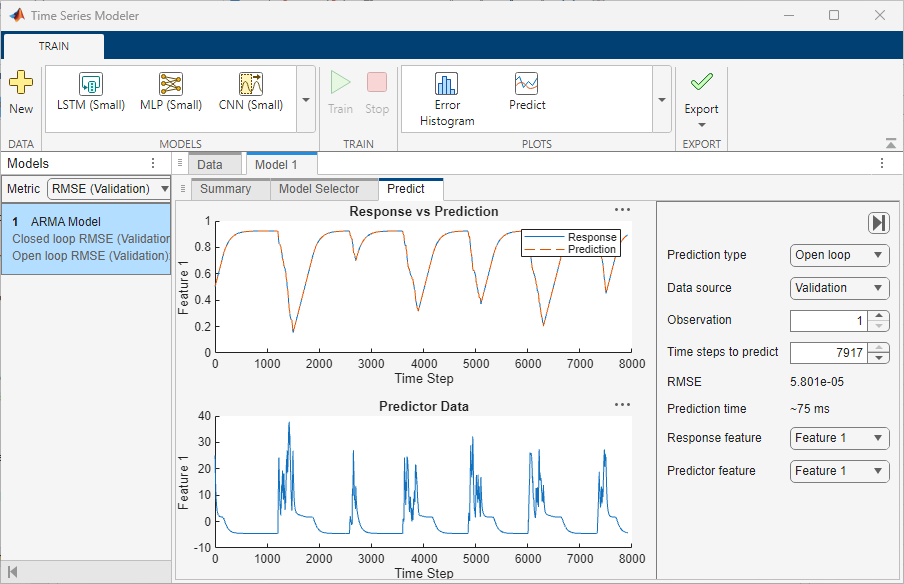
Model Selector tab displaying the generated candidate models in the app

Predict Values for Data

On the toolstrip, click Predict. The Predict tab opens. To use the selected model to predict values for the training and validation data and view plots of the results, set these options:

Prediction type — Select the type of prediction as Closed loop or Open loop. For more information, see the open loop and closed loop table under the Model Selection section.
Data source — Select whether to predict on the training data or the validation data. The performance of the model on the validation data is usually a more accurate reflection of how the model will perform on new data.
Observation — Enter the experiment number of the data for which you want to predict values.
Time steps to predict — The app reserves the first few samples from the data set (n₁) to compute the initial conditions. It uses the rest of the samples (n₂<=N-n₁) to compute the predicted response and compare it to the corresponding measured values. Use the Time steps to predict option to specify the value of n₂.
Response feature — Select the response feature whose predicted values you want to view. This option is useful if the imported data includes multiple outputs.
Predictor feature — Select the predictor feature to view. This option is useful if the imported data includes multiple inputs.

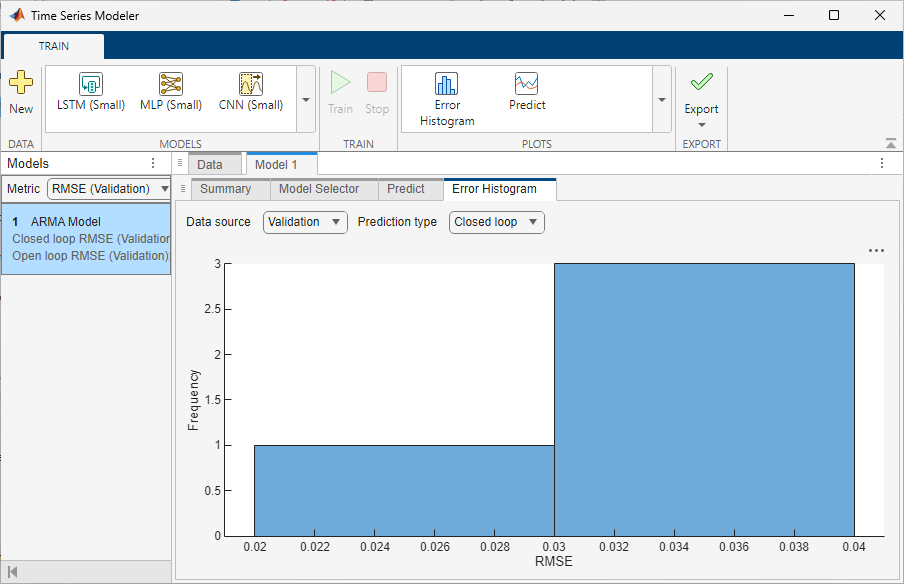
The app displaying response vs prediction plots on the Predict tab

Plot Error Histogram

To plot a histogram of the RMSE errors for either the training or validation data, on the toolstrip, click Error Histogram. The Error Histogram tab opens. Set these options:

Prediction type — Select the type of prediction as Closed loop or Open loop. For more information, see the open loop and closed loop table under the Model Selection section.
Data source — Select whether to predict on the training data or the validation data. The performance of the model on the validation data is usually a more accurate reflection of how the model will perform on new data.

The error histogram plot is only available if you have multiple observations, that is, multiple experiments.

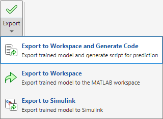
The app displaying the error histogram

Export Trained Model

To export the trained model and the training statistics to the MATLAB workspace and generate a live script for predicting on new data, on the toolstrip, click Export. The app exports a structure that contains an idpoly model and generates a live script that contains code for preparing and predicting values for new data.

To only export the trained model to the MATLAB workspace and not generate code, click Export > Export to Workspace. The app exports a structure that contains an idpoly model.

To export the trained model to Simulink^® as an Idmodel block, click Export > Export to Simulink. The Export to Simulink dialog box opens. In this dialog box, you can choose to export the trained model as one of these model types:

Simulation model — The generated Idmodel block has only one input port for injecting input signals.
Finite-horizon prediction model — The generated Idmodel block has two input ports, one for injecting input signals and one for injecting the measured output values. In the Export to Simulink dialog box, you specify Horizon (number of steps) as a positive integer.

You can also specify the folder in which the app will save the Simulink model. By default, the app saves the model in the current working folder.

Export options in the app