Reduced Order Modeling of Electric Vehicle Battery System Using Neural State-Space Model

Generate Synthetic Training and Validation Data Sets from High-Fidelity Simscape Model

As a data-driven modeling approach, reduced order modeling using deep networks leverages the massive amount of data available from connected devices and sensors, and the key to success heavily relies on the quality and quantity of the training data set. Therefore, you need to carefully devise the design of experiments (DOE) such that the design space, including the state space and control action space, is traversed sufficiently by manipulating initial conditions and input signals. In this example, you train the neural state-space model with synthetic data sets generated from the high-fidelity model in Simulink, while you generate the validation data set from the same model under a highway drive cycle current profile. Alternatively, you can generate the training and validation data sets from physical equipment in a laboratory. In this example, you devise the DOE carefully to cover the four-dimensional design space including the state of charge (SOC), current, voltage, and temperature. To sample the design space and provide a uniform coverage, use the Sobol sequence method.

First, add the Data and Models folders to the MATLAB® path.

addpath('./Data');
addpath('./Models');

For this example, load previously saved training and validation data sets into the MATLAB workspace. To reduce the size of the MAT file, store these data sets in single precision using different variables.

Alternatively, to generate new data sets, set UseSavedDataSets to false in the code below. To learn how the Sobol sequences are designed and injected into the high-fidelity models to traverse the design space, open the SyntheticDataGeneration.m file. You call this function to generate synthetic data sets from simulation. The simulation takes a few minutes to complete.

UseSavedDataSets = true; 
if UseSavedDataSets
   load TrainingValidationData.mat;
   BattInputs_Train = double(BattInputs_Train);
   BattInputs_Validation = double(BattInputs_Validation);
   BattOutputs_Train = double(BattOutputs_Train);
   BattOutputs_Validation = double(BattOutputs_Validation);   
else
   [BattInputs_Train,BattOutputs_Train,BattInputs_Validation,BattOutputs_Validation] = SyntheticDataGeneration; 
end

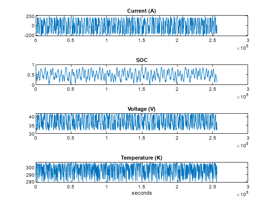
Examine the training data set, which is a very long experiment taking more than 70 hours. Data is logged at a sampling rate of 2 seconds.

figure; tiledlayout(4,1)
times_training = (0:size(BattInputs_Train,1)-1)*2;
ax1 = nexttile; plot(times_training,BattInputs_Train(:,1)); title('Current (A)');
ax2 = nexttile; plot(times_training,BattInputs_Train(:,2)); title('SOC');
ax3 = nexttile; plot(times_training,BattOutputs_Train(:,1)); title('Voltage (V)');
ax4 = nexttile; plot(times_training,BattOutputs_Train(:,2)); title('Temperature (K)');
xlabel('seconds');
linkaxes([ax1 ax2 ax3 ax4],'x');

Examine the validation data set, which is generated based on a standard highway drive current profile in about 18 minutes.

figure; tiledlayout(4,1)
times_validation = (0:size(BattInputs_Validation,1)-1)*2;
ax1 = nexttile; plot(times_validation,BattInputs_Validation(:,1)); title('Current (A)');
ax2 = nexttile; plot(times_validation,BattInputs_Validation(:,2)); title('SOC');
ax3 = nexttile; plot(times_validation,BattOutputs_Validation(:,1)); title('Voltage (V)');
ax4 = nexttile; plot(times_validation,BattOutputs_Validation(:,2)); title('Temperature (K)');
xlabel('seconds');
linkaxes([ax1 ax2 ax3 ax4],'x');

Train Neural State-Space Model

Depending on your use case, you can apply several optional data preprocessing techniques to the original experiment data to help make training converge faster and its result more reliable. In this example, you normalize the state and input data with the mean and standard deviation such that they have relatively the same order of magnitude. Then you obtain trajectories for them.

mu_input = mean(BattInputs_Train);
sig_input = std(BattInputs_Train);
mu_output = mean(BattOutputs_Train);
sig_output = std(BattOutputs_Train);

BattInputs_Train = (BattInputs_Train - mu_input)./sig_input;
BattOutputs_Train = (BattOutputs_Train - mu_output)./sig_output;
BattInputs_Validation = (BattInputs_Validation - mu_input)./sig_input;
BattOutputs_Validation = (BattOutputs_Validation - mu_output)./sig_output;

current_train = BattInputs_Train(:,1);
soc_train = BattInputs_Train(:,2);
voltage_train = BattOutputs_Train(:,1);
temperature_train = BattOutputs_Train(:,2);
current_validation = BattInputs_Validation(:,1);
soc_validation = BattInputs_Validation(:,2);
voltage_validation = BattOutputs_Validation(:,1);
temperature_validation = BattOutputs_Validation(:,2);

The duration of a trajectory defined in a training data set is important for network training. During the training process, the algorithm compares the error between the estimated data points and the measured data points along the predicted trajectory. If the duration is too long, the modeling error is amplified and a larger error accumulates at the later prediction steps, which makes training more difficult. If the duration is too small, you have too many training data sets, which significantly slows down the training process. In this example, you split the original 70-hour long experiment into N (about 5100) segments, such that each data set used in training has 25 prediction steps (equivalent to duration of 50 seconds), and save them as cell arrays of timetables. Due to the nature of state-space trajectories, you can use any time point in the long experiment as the starting point of a training data set.

PredictionSteps = 25;
N = round(length(current_train)/PredictionSteps)-1;
time_vector = seconds(0:2:2*PredictionSteps);
for ct=1:N
   tmp = array2timetable(current_train((ct-1)*PredictionSteps+1:ct*PredictionSteps+1,:),"RowTimes",time_vector);
   tmp.Properties.VariableNames = {'Current'};
   CurrentArray{ct} = tmp; 

   tmp = array2timetable(soc_train((ct-1)*PredictionSteps+1:ct*PredictionSteps+1,:),"RowTimes",time_vector);
   tmp.Properties.VariableNames = {'SOC'};
   SOCArray{ct} = tmp;

   tmp = array2timetable(voltage_train((ct-1)*PredictionSteps+1:ct*PredictionSteps+1,:),"RowTimes",time_vector);
   tmp.Properties.VariableNames = {'Voltage'};
   VoltageArray{ct} = tmp;

   tmp = array2timetable(temperature_train((ct-1)*PredictionSteps+1:ct*PredictionSteps+1,:),"RowTimes",time_vector);
   tmp.Properties.VariableNames = {'Temperature'};
   TemperatureArray{ct} = tmp;
end

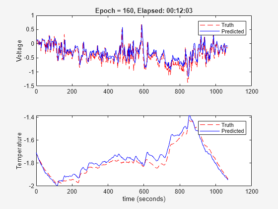
To validate the training result, use the whole validation experiment as the validation data set to see whether the trained neural state-space model can achieve good prediction results even when the validation data set duration (18 minutes) is much longer than the training data set duration (50 seconds).

len = length(current_validation);
time_vector = seconds(0:2:2*(len-1));
Current_Validation = array2timetable(current_validation,"RowTimes",time_vector);
Current_Validation.Properties.VariableNames = {'Current'};
SOC_Validation = array2timetable(soc_validation,"RowTimes",time_vector);
SOC_Validation.Properties.VariableNames = {'SOC'};
Voltage_Validation = array2timetable(voltage_validation,"RowTimes",time_vector);
Voltage_Validation.Properties.VariableNames = {'Voltage'};
Temperature_Validation = array2timetable(temperature_validation,"RowTimes",time_vector);
Temperature_Validation.Properties.VariableNames = {'Temperature'};

You need to assemble the data sets into the input arguments U and Y, as required by the training command nlssest. The first N entries in U and Y are training data sets and the last entries are used for validation.

for ct = 1:N
   Y{ct} = [VoltageArray{ct} TemperatureArray{ct}];
   U{ct} = [CurrentArray{ct} SOCArray{ct}];
end
Y{N+1} = [Voltage_Validation Temperature_Validation];
U{N+1} = [Current_Validation SOC_Validation];

To train a new model, create a neural state-space object using idNeuralStateSpace, specify an MLP network for the state function, specify training options, and train the neural network with the validation plot. Training the model takes about 10 minutes. To reproduce training results consistently, use a seed for random number generation before training.

Alternatively, for the sake of example efficiency, load a previously trained neural state-space model into the MATLAB workspace by setting UseSavedNSS to true in the code below.

rng(0); 
UseSavedNSS = false;
if UseSavedNSS
   load TrainedNSSModel.mat;
else
   Ts = 2;  
   obj = idNeuralStateSpace(2,NumInputs=2,Ts=Ts);
   obj.StateNetwork = createMLPNetwork(obj,'state', ...
      LayerSizes=[128 128], ...
      Activations='tanh', ...
      WeightsInitializer="glorot", ...
      BiasInitializer="zeros");
   options = nssTrainingOptions('adam');
   options.MaxEpochs = 160;
   options.MiniBatchSize = 200; 
   options.LearnRate = 0.0002;
   obj = nlssest(U,Y,obj,options,UseLastExperimentForValidation=true,ValidationFrequency=5);
end

Generating estimation report...done.

Validate Neural State-Space Model Performance in Simulink

To predict voltage and temperature, use the trained neural state-space model in a Neural State-Space Model block in Simulink. Load the current profile with normalized data and simulate the model. Compare the Simscape model simulation results against the neural state-space model prediction results of the surrogate model in Simulink under a dynamic drive cycle current profile.

[mu_input,sig_input,mu_output,sig_output,BattOutputs_Validation] = DataNormalization; 

cd Models
open_system("ValidationModel_Simscape_NSS");
out = sim('ValidationModel_Simscape_NSS.slx');

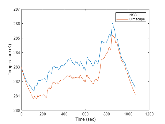
Compare temperature trajectories by plotting the neural state-space predicted temperature followed by the Simscape simulated temperature.

figure; 
plot(out.logsout{1}.Values.Time,out.logsout{1}.Values.Data(:));
hold on; plot(out.logsout{3}.Values.Time,out.logsout{3}.Values.Data(:)); 
xlabel('Time (sec)'); ylabel('Temperature (K)');
legend({'NSS','Simscape'}); 

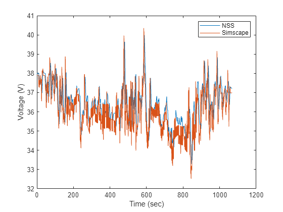
Compare voltage trajectories by plotting the neural state-space predicted voltage followed by the Simscape simulated voltage.

figure; 
plot(out.logsout{2}.Values.Time,out.logsout{2}.Values.Data(:));
hold on; plot(out.logsout{4}.Values.Time,out.logsout{4}.Values.Data(:));
xlabel('Time (sec)'); ylabel('Voltage (V)');
legend({'NSS','Simscape'});

As shown in the plots, the voltage and temperature trajectories predicted by the neural state-space model (NSS) match the trajectories generated by the high-fidelity Simscape model very well.

Finally, remove the Data and Models folders from the MATLAB path.

cd ..
rmpath('./Data');
rmpath('./Models');

Copyright 2023 The MathWorks, Inc.