2-D Finite Impulse Response (FIR) Filters

Image Processing Toolbox™ supports only one class of linear filter: the two-dimensional finite impulse response (FIR) filter. All of the Image Processing Toolbox filter design functions return FIR filters.

FIR filters have several characteristics that make them ideal for image processing in MATLAB^®.

You can design 2-D FIR filters for image processing using various methods. These examples show how to create a 2-D low-pass FIR filter using three different methods. Each method uses a different form of approximation, and thus the outputs of the three methods differ to some extent.

Design 2-D FIR Filter Using Frequency Sampling Method

This example shows how to design a 2-D FIR filter using the frequency sampling method on a desired frequency response.

Given a matrix that defines the shape of the frequency response, the frequency sampling method creates a filter in the spatial domain whose frequency response matches the matrix at the sampled frequencies. Frequency sampling places no constraints on the behavior of the frequency response of the filter between the sampled frequencies. Further, frequency sampling might not be able to capture discontinuities in the ideal frequency response. These interpolation errors and discontinuities usually cause ripples in the frequency response of the filter. Ripples are oscillations around a constant value. The frequency response of a practical filter often has ripples, whereas the frequency response of an ideal filter is flat.

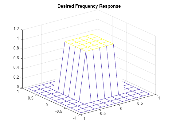
Define and visualize the target 2-D frequency response of an 11-by-11 filter.

Hd = zeros(11,11); 
Hd(4:8,4:8) = 1;
[f1,f2] = freqspace(11,"meshgrid");
mesh(f1,f2,Hd)
title("Desired Frequency Response")

Create the filter based on the target frequency response using the fsamp2 function. The fsamp2 function returns the filter h in the spatial domain with a frequency response that passes through the points in the input matrix Hd.

h = fsamp2(Hd);

Plot the frequency response of the filter.

freqz2(h,[32 32])
title("Actual Frequency Response")

Notice the ripples in the actual frequency response compared to the desired frequency response. These ripples are a fundamental problem with the frequency sampling design method that occur wherever there are sharp transitions in the desired response. You can reduce the spatial extent of the ripples by using a larger filter. However, a larger filter does not reduce the height of the ripples, and requires more computation time for filtering. To achieve a smoother approximation of the desired frequency response, consider using the frequency transformation method or the windowing method, instead.

Filter an image using the designed filter, and visualize the results.

inputImage = imread("coins.png");
outputImage = imfilter(inputImage,h);
imshowpair(inputImage,outputImage,"montage")

Design 2-D FIR Filter Using Frequency Transformation Method

This example shows how to design a 2-D FIR filter using the frequency transformation method on a 1-D FIR filter.

Given a 1-D FIR filter with particular characteristics, the frequency transformation method creates a corresponding 2-D FIR filter preserving most of the characteristics of the 1-D filter, particularly the transition bandwidth and ripple characteristics. The shape of the 1-D frequency response is clearly evident in the 2-D frequency response. This method uses a transformation matrix, a set of elements that defines the frequency transformation.

Define a 1-D FIR filter using the firpm (Signal Processing Toolbox) function.

b = firpm(10,[0 0.4 0.6 1],[1 1 0 0])

b = 1×11

    0.0537   -0.0000   -0.0916   -0.0001    0.3131    0.4999    0.3131   -0.0001   -0.0916   -0.0000    0.0537

Plot the frequency response of the 1-D filter.

[H,w] = freqz(b,1,64,"whole");
plot(w/pi-1,fftshift(abs(H)))
title("One-Dimensional Frequency Response")

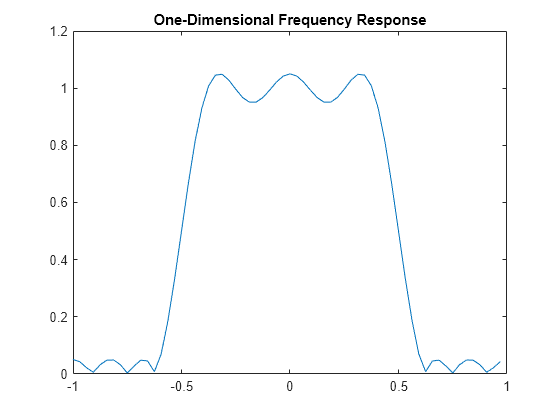
Transform the 1-D filter into a 2-D filter using the ftrans2 function. The default transformation matrix of the ftrans2 function produces filters with nearly circular symmetry. By defining your own transformation matrix, you can obtain different symmetries.

h = ftrans2(b);

Plot the frequency response of the 2-D filter.

freqz2(h,[32 32])
title("Corresponding Two-Dimensional Frequency Response")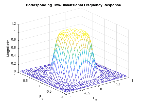

Filter an image using the designed filter, and visualize the results.

inputImage = imread("coins.png");
outputImage = imfilter(inputImage,h);
imshowpair(inputImage,outputImage,"montage")

Design 2-D FIR Filter Using Windowing Method

This example shows how to design a 2-D FIR filter using the windowing method on a desired frequency response.

Given a matrix that defines the shape of the frequency response, the windowing method creates a filter in the spatial domain that is the product of the desired impulse response and a tapering window function. Like the frequency sampling method, the windowing method produces a filter whose frequency response approximates a desired frequency response. The windowing method, however, tends to produce better results than the frequency sampling method as it reduces discontinuities and interpolation errors, resulting in less intense ripples.

Define and visualize the target 2-D frequency response of an 11-by-11 filter.

Hd = zeros(11,11);
Hd(4:8,4:8) = 1;
[f1,f2] = freqspace(11,"meshgrid");
mesh(f1,f2,Hd)
axis([-1 1 -1 1 0 1.2])
title("Desired Frequency Response")

You can define a 2-D window by specifying a 2-D window directly using the fwind2 function, or by converting one or two 1-D windows into a two-dimensional window using the fwind1 function. If you specify a single 1-D window, fwind1 transforms the 1-D window using a process similar to rotation, resulting in a 2-D window with near circular symmetry. If you specify two 1-D windows, fwind1 computes their outer product, making the 2-D window rectangular and separable.

Specify a single 1-D Hamming window using the hamming (Signal Processing Toolbox) function.

win1d = hamming(11);

Create an 11-by-11 filter from the desired frequency response Hd and the 1-D window.

h = fwind1(Hd,win1d);

Plot the frequency response of the filter.

freqz2(h,[32 32])
axis([-1 1 -1 1 0 1.2])
title("Actual Frequency Response")

Filter an image using the designed filter, and visualize the results.

inputImage = imread("coins.png");
outputImage = imfilter(inputImage,h);
imshowpair(inputImage,outputImage,"montage")