识别植被和非植被频谱
此示例说明如何:
使用二维频谱数据作为高光谱函数的超立方。
使用
ndvi函数分离植被和非植被频谱。
此示例需要 Image Processing Toolbox™ 的 Hyperspectral Imaging Library。您可以从附加功能资源管理器安装 Image Processing Toolbox 的 Hyperspectral Imaging Library。有关安装附加功能的详细信息,请参阅获取和管理附加功能。Image Processing Toolbox 的 Hyperspectral Imaging Library 需要桌面 MATLAB®,因为 MATLAB® Online™ 和 MATLAB® Mobile™ 不支持该库。
加载二维频谱数据
将包含 Indian Pines 数据集的 20 个端元的二维频谱数据加载到工作区中。
load("indian_pines_endmembers_20.mat")将 Indian Pines 数据集的每个频带的波长值加载到工作区中。
load("indian_pines_wavelength.mat")准备用于高光谱函数的测试数据
使用 reshape 函数将二维频谱数据重构为三维体数据。
[numSpectra,spectralDim] = size(endmembers);
dataCube = reshape(endmembers,[numSpectra 1 spectralDim]);
通过将三维体数据 dataCube 和波长信息 wavelength 指定给 hypercube 函数,创建一个具有单一维度的三维 hypercube 对象。
hcube = imhypercube(dataCube,wavelength);
计算 NDVI 以分离植被和非植被频谱
计算超立方对象中每个频谱的 NDVI 值。
ndviVal = ndvi(hcube);
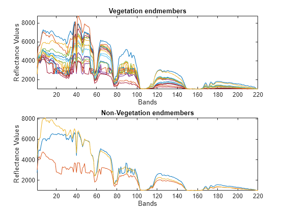
植被频谱通常具有大于零的 NDVI 值,而非植被频谱通常具有小于零的 NDVI 值。执行阈值化以分离植被和非植被频谱。
index = ndviVal > 0;
绘制植被和非植被端元。
subplot(2,1,1)
plot(endmembers(index,:)')
title("Vegetation endmembers")
xlabel("Bands")
ylabel("Reflectance Values")
axis tight
subplot(2,1,2)
plot(endmembers(~index,:)')
title("Non-Vegetation endmembers")
xlabel("Bands")
ylabel("Reflectance Values")
axis tight
另请参阅
hypercube | spectralMatch | ndvi