Process Large Hyperspectral Images

Download Data Set

Download and unzip the data set. The total size of the data set is approximately 7GB. The download may take a long time depending on your internet connection.

zipFile = matlab.internal.examples.downloadSupportFile("image","data/f140826t01p00r08rdn_b.zip");
filepath = fileparts(zipFile);
unzip(zipFile,filepath)

Load and Visualize Small Region of the Large Hyperspectral Data

Load the hyperspectral data into the workspace as a hypercube object. Note that the size of the hyperspectral image is 27068-by-1302-by-224 which would require a large amount of system memory to load at once. However, because the hypercube function loads only the metadata of the hyperspectral data into the workspace, rather than the hyperspectral datacube, MATLAB does not return an out of memory error despite the size of the hyperspectral image.

filename = fullfile(filepath,"f140826t01p00r08rdn_b","f140826t01p00r08rdn_b_sc01_ort_img");
hcube = hypercube(filename)

hcube = 
  hypercube with properties:

      DataCube: "[27068x1302x224 int16]"
    Wavelength: [224×1 double]
      Metadata: [1×1 struct]

Crop the hyperspectral image to get a 3001-by-1302-by-224 hyperspectral image.

hcube = cropData(hcube,22000:25000,":")

hcube = 
  hypercube with properties:

      DataCube: "[3001x1302x224 int16]"
    Wavelength: [224×1 double]
      Metadata: [1×1 struct]

Remove every band after the first 100 spectral bands to reduce the size of the hyperspectral image to 3001-by-1302-by-100.

hcube = removeBands(hcube,BandNumber=151:224)

hcube = 
  hypercube with properties:

      DataCube: "[3001x1302x150 int16]"
    Wavelength: [150×1 double]
      Metadata: [1×1 struct]

Create and visualize an RGB representation of the cropped hyperspectral image.

rgbImg = colorize(hcube,Method="rgb",ContrastStretching=true);
figure
imshow(rgbImg)

Compute Custom Water Index on Cropped Hyperspectral Image

You can use the wavelengths in the green band and the short-wave infrared (SWIR) band to estimate the position of a water body in the cropped hyperspectral image. The range of wavelengths in the green band is 500–600 nm, while the range of wavelengths in the SWIR band is 1550–1750 nm. Find the wavelengths in the cropped hyperspectral image closest to the midpoints of the green band and the SWIR band.

[~,greenIdx] = min(abs(hcube.Wavelength-550));
[~,swirIdx] = min(abs(hcube.Wavelength-1650));
wavelengths = [hcube.Wavelength(greenIdx) hcube.Wavelength(swirIdx)];

Create a function handle for a custom spectral index formula that estimates a water body from the green band and SWIR band wavelengths.

func = @(green,swir) (green-swir)./(green+swir);

Apply the custom water estimation formula to the cropped hyperspectral image to get the water body index image.

waterImg = customSpectralIndex(hcube,wavelengths,func);

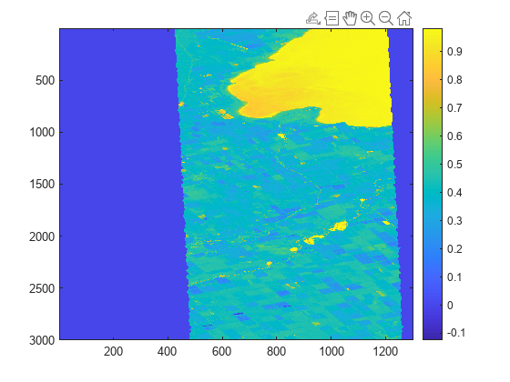
Visualize the water body index image. The index indicates the likelihood that the location represented by a given pixel is part of a body of water, with higher values indicating a greater probability.

figure
imagesc(waterImg)
colorbar

Compute NDVI on Cropped Hyperspectral Image

Compute the normalized difference vegetation index (NDVI) on the cropped hyperspectral image.

ndviImg = ndvi(hcube);

Visualize the NDVI image. The index indicates the likelihood that the location represented by a given pixel has vegetation, with higher values indicating a greater probability.

figure
imagesc(ndviImg)
colorbar