Export Point Cloud Segmentations to KML Files

This example uses:

This example shows how to export segmented point cloud data to a Keyhole Markup Language (KML) files and read and visualize the KML data using different tools.

KML is an XML-based markup language designed for visualizing geographic data on web-based maps or Earth browsers, such as Google Earth™, Google Maps™, NASA WorldWind, and the Esri® ArcGIS™ Explorer. The KML international standard is maintained by the Open Geospatial Consortium, Inc. (OGC).

Load and Visualize Point Cloud Data

This example uses the point cloud data from the LAS file aerialLidarData2.las, obtained from the Open Topography Dataset [1]. Load the point cloud data into the workspace using the readPointCloud function of the lasFileReader object,and visualize the point cloud.

% Specify the LAS file path
lasfile = fullfile(toolboxdir("lidar"),"lidardata","las", ...
    "aerialLidarData2.las");

% Create a lasFileReader object
lasReader = lasFileReader(lasfile);

% Read the point cloud
ptCloud = readPointCloud(lasReader);

% Visualize the point cloud
figure
pcshow(ptCloud)
axis on
title("Input Aerial Lidar Data")

Figure contains an axes object. The axes object with title Input Aerial Lidar Data contains an object of type scatter.

Segment Point Cloud Data

This example segments the point cloud into buildings and vegetation by using a feature-based classification algorithm. First, perform ground segmentation by using the segmentGroundSMRF function, and then classify the nonground points into vegetation and building by using the helperSegment helper function.

% Segment the point cloud into ground and nonground points
[groundIdx,nonGroundPtCloud,groundPtCloud] = segmentGroundSMRF(ptCloud);

Segment the nonground point cloud into vegetation and buildings by using the helperSegment helper function, defined at the end of this example.

% Store the labels for each point in clusterLabels. 
% Label 1 : Ground, 
% Label 2 : Vegetation,
% Label 3 : Building
clusterLabels = ones(ptCloud.Count,1);

% Segment the vegetation and buildings from the nonground point cloud
labels = helperSegment(nonGroundPtCloud);
clusterLabels(~groundIdx) = labels;

% Compute the indices of the vegetation and building points in the point cloud
vegetationIdx = clusterLabels == 2;
buildingIdx = clusterLabels == 3;

Next, cluster the individual trees from the vegetation point cloud by using the helperClusterVeg helper function, attached to this example as a supporting file.

% Extract the vegetation point cloud from the input point cloud
vegPtCloud = select(ptCloud,vegetationIdx);

% Specify the grid size (in meters per pixel)
gridRes = 2;

% Specify the minimum tree height (in meters)
minTreeHeight = 5;

% Cluster the individual trees from the segmented vegetation point cloud
[validIds,vegClusterLabels] = helperClusterVeg(groundPtCloud, ...
    vegPtCloud,gridRes,minTreeHeight);

% Create a logical array of the vegetation points in the clusters
clusterVegetationIdx = vegetationIdx;
vegetationInd = find(clusterVegetationIdx);
clusterVegetationIdx(vegetationInd(~validIds)) = false;

Cluster the individual buildings from the building point cloud by using the pcsegdist function.

% Extract the building point cloud from the input point cloud
buildingPtCloud = select(ptCloud,buildingIdx);

% Cluster the individual buildings from the segmented building point cloud
minDistance = 2;
buildingClusterLabels = pcsegdist(buildingPtCloud,minDistance, ...
    NumClusterPoints=10);

Write Point Cloud Data to KML

To write point cloud data to a KML file, you must first convert the point cloud segmentations into real-world locations. This conversion requires a coordinate reference system (CRS). A CRS provides a framework for defining real-world locations. You can describe geographic data using these types of CRSs:

Geographic Coordinate Reference System — Provides information that assigns latitude, longitude, and height coordinates to real-world locations. A geographic CRS consists of a datum, a prime meridian, and an angular unit of measurement. To know more about geographic CRSs, see the geocrs (Mapping Toolbox) object.
Projected Coordinate Reference System — Provides information that assigns Cartesian x- and y- coordinates to real-world locations. A projected CRS consists of a geographic CRS and several other parameters to transform coordinates to and from the geographic CRS. To know more about projected CRSs, see the projcrs (Mapping Toolbox) object.

This example uses the projected CRS data from the LAS file to convert the point cloud segmentations to real-world locations. To check if the LAS file contains the projected CRS data, use the hasCRSData function of the lasFileReader object.

Extract the projected CRS data from the LAS file using the readCRS function of the lasFileReader object. Then, extract the x- and y- coordinates of the point cloud segmentations. Use inverse projection with the projected CRS data to compute latitude and longitude data from these x- and y- coordinates. Write the point cloud data to a KML file by using the kmlwritepoint (Mapping Toolbox) function.

% Read the CRS data
projCRSData = readCRS(lasReader);

% Convert the point cloud x- and y-coordinates to latitude and longitude
[lat,lon] = projinv(projCRSData,ptCloud.Location(:,1), ...
    ptCloud.Location(:,2));

% Extract the heights of the points
altitude = ptCloud.Location(:,3);

% Write data to KML files
kmlwritepoint("Building.kml",lat(buildingIdx),lon(buildingIdx), ...
    altitude(buildingIdx));
kmlwritepoint("Vegetation.kml",lat(vegetationIdx), ...
    lon(vegetationIdx),altitude(vegetationIdx));

Read KML Data

Read the Building.kml and Vegetation.kml files into the workspace as geospatial tables by using the readgeotable (Mapping Toolbox) function.

% Read the KML files
buildingKMLData = readgeotable("Building.kml");
vegetationKMLData = readgeotable("Vegetation.kml");

Visualize KML Data

There are several ways to visualize the KML data. In this example, you will visualize the data on a map, on a globe, and using RoadRunner.

On A Map

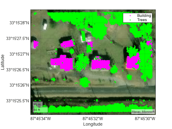
Visualize the data read from the KML files by using the geoplot (Mapping Toolbox) function.

figure
geoplot(buildingKMLData,MarkerEdgeColor="magenta")
hold on
geoplot(vegetationKMLData,MarkerEdgeColor="green")
hold off
geobasemap satellite
legend("Building","Trees")

Figure contains an axes object with type geoaxes. The geoaxes object contains 2 objects of type point. These objects represent Building, Trees.

On A Globe

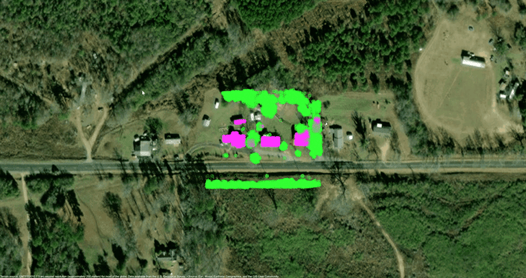
Use the geoglobe (Mapping Toolbox) function, to visualize the data on a globe.

g = geoglobe(uifigure);
geoplot3(g,buildingKMLData.Shape.Latitude,buildingKMLData.Shape.Longitude, ...
    altitude(buildingIdx),"mo")
hold(g,"on")
geoplot3(g,vegetationKMLData.Shape.Latitude,vegetationKMLData.Shape.Longitude, ...
    altitude(vegetationIdx),"go")
hold(g,"off")

% Set the camera height
camheight(g,5*max(altitude))

Using RoadRunner

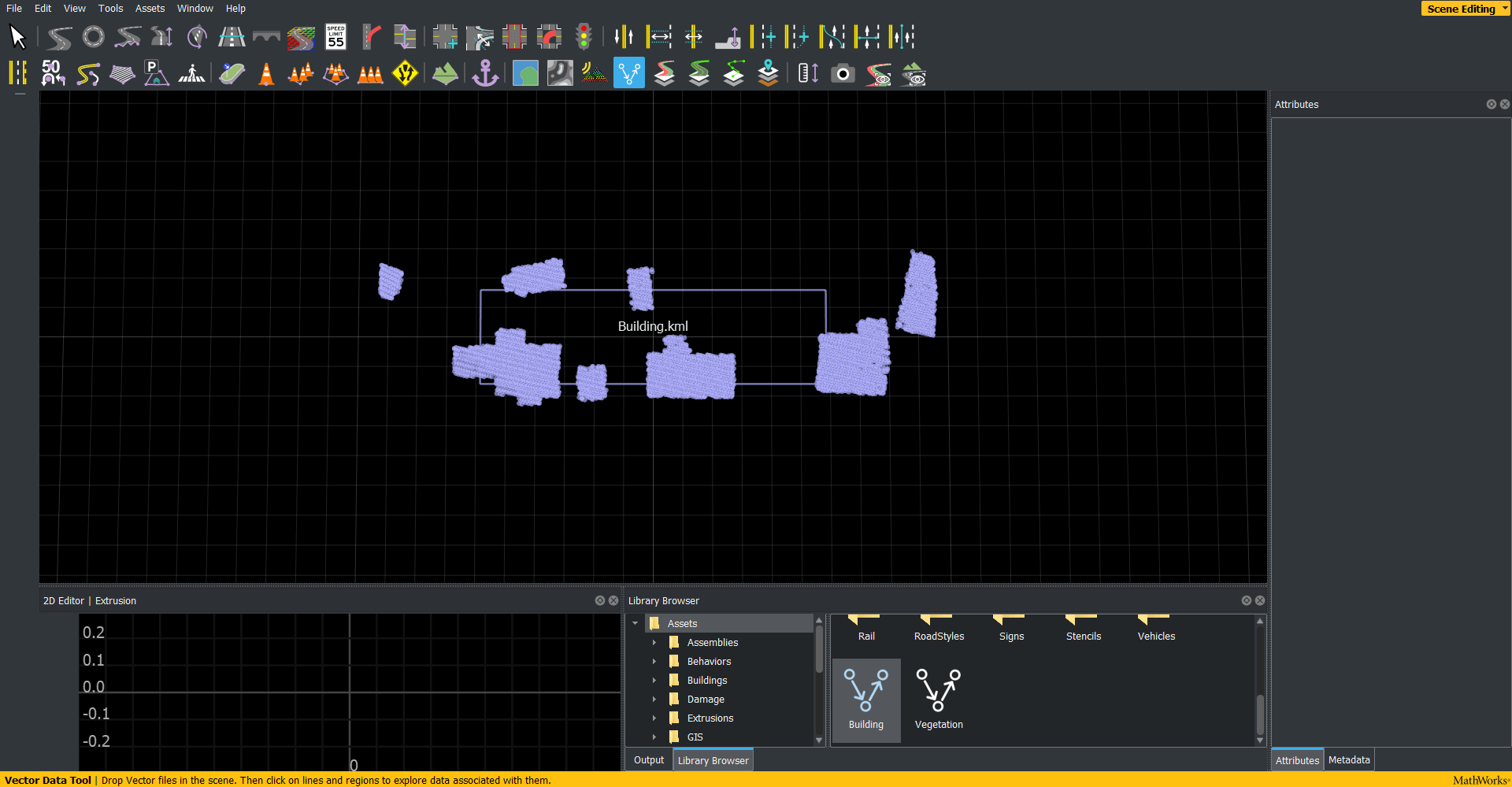
To visualize the data using RoadRunner, you must first import the KML data into RoadRunner, using the Vector Data Tool. You can also add color to the KML data.

Follow these steps to import the Building.kml file into RoadRunner.

1) Import the Building.kml file into RoadRunner by using the Vector Data Tool.

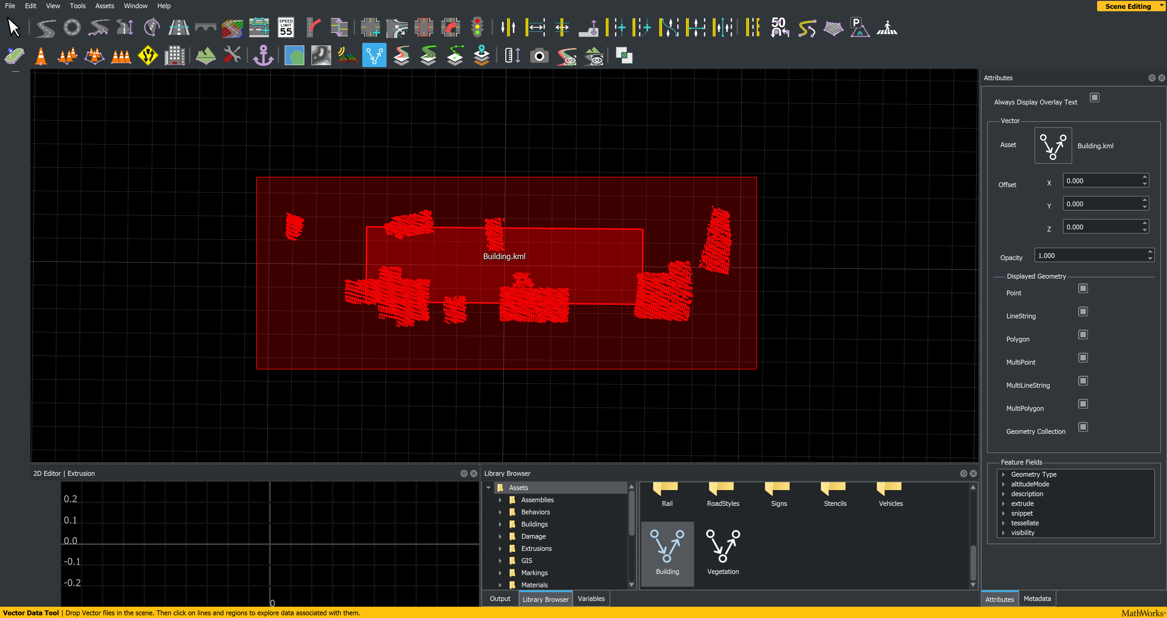
2) Select the data you want to add color to.

3) In the Attributes pane, right-click Geometry Type, and select Color With.

4) Choose the color from the available options.

Repeat this process for the vegetation and visualize the results.

Note: You cannot write or access the color data of a KML file using RoadRunner. You must add colors every time you import the KML data into RoadRunner.

Helper Functions

The helperSegment helper function segments buildings and vegetation from a nonground point cloud. For more details on this workflow, see the Terrain Classification for Aerial Lidar Data example.

function labels = helperSegment(nonGroundPtCloud)
% Specify the number of neighbors
neighbors = 10;

% Extract the normal and curvature features
[normals,curvatures,neighInds] = helperExtractFeatures(nonGroundPtCloud, ...
    neighbors);

% Specify the normal threshold and curvature threshold
normalThresh = 0.75;
curveThresh = 0.035;

% Classify the point cloud into vegetation and buildings
%     Class    |  Label id
%   Vegetation |   2
%   Building   |   3
labels = helperClassify(normals,curvatures,neighInds, ...
    normalThresh,curveThresh);
labels = labels+1;
end

References

[1] Starr, Scott. "Tuscaloosa, AL: Seasonal Inundation Dynamics and Invertebrate Communities." National Center for Airborne Laser Mapping, December 1, 2011. OpenTopography. https://doi.org/10.5069/G9SF2T3K.