Main Content

lte3DChannel

Filter signal through 3-D MIMO fading channel

Description

The lte3DChannel System object™ filters an input signal through the TR 36.873 link-level multiple-input/multiple-output (MIMO) fading channel to obtain the channel-impaired signal. The object implements these channel processing steps defined in TR 36.873 [1], Section 7.3:

  • Step 7: Adding ray offset angles

  • Step 8: Coupling of rays

  • Step 9: Generating cross-polarization power ratios (XPRs)

  • Step 10: Drawing random initial phases

  • Step 11: Generating channel coefficients for each cluster

To filter an input signal using the TR 36.873 link-level MIMO fading channel:

  1. Create the lte3DChannel object and set its properties.

  2. Call the object with arguments, as if it were a function.

To learn more about how System objects work, see What Are System Objects?

Creation

Description

lte3d = lte3DChannel creates a TR 36.873 link-level MIMO System object.

lte3d = lte3DChannel(Name,Value) creates the object with properties set by using one or more name-value pairs. Enclose the property name inside quotes, followed by the specified value. Unspecified properties take default values.

Example: lte3d = lte3DChannel('PathDelays',2e-6,'HasLOSCluster',true,'KFactorFirstCluster',12) creates the channel object with a path delay of two microseconds, the LOS cluster of the delay profile enabled, and a K-factor of 12 dB for the first cluster of the delay profile.

example

lte3d = lte3DChannel.makeCDL(DelayProfile) creates the object with the specified CDL delay profile from TR 38.901 [2] Section 7.7.1, and a delay spread of 30 ns.

example

lte3d = lte3DChannel.makeCDL(DelayProfile,DelaySpread) creates the object with the specified CDL delay profile and delay spread.

example

lte3d = lte3DChannel.makeCDL(DelayProfile,DelaySpread,KFactor) creates the object with the specified CDL delay profile, delay spread, and K-factor scaling.

Input Arguments

expand all

Delay profile, specified as one of 'CDL-A', 'CDL-B', 'CDL-C', 'CDL-D', or 'CDL-E'.

Delay spread in ns, specified as a numeric scalar.

Data Types: double

K-factor scaling, specified as a numeric scalar. K-factor scaling applies only when you specify DelayProfile as 'CDL-D' or 'CDL-E'.

Data Types: double

Properties

expand all

Unless otherwise indicated, properties are nontunable, which means you cannot change their values after calling the object. Objects lock when you call them, and the release function unlocks them.

If a property is tunable, you can change its value at any time.

For more information on changing property values, see System Design in MATLAB Using System Objects.

Discrete path delays in seconds, specified as a numeric scalar or row vector. AveragePathGains and PathDelays must have the same size.

Data Types: double

Average path gains in dB, specified as a numeric scalar or row vector. AveragePathGains and PathDelays must have the same size.

Data Types: double

Azimuth of arrival angle in degrees, specified as a numeric scalar or row vector. The vector elements specify the angles for each cluster.

Data Types: double

Azimuth of departure angle in degrees, specified as a numeric scalar or row vector. The vector elements specify the angles for each cluster.

Data Types: double

Zenith of arrival angle in degrees, specified as a numeric scalar or row vector. The vector elements specify the angles for each cluster.

Data Types: double

Zenith of departure angle in degrees, specified as a numeric scalar or row vector. The vector elements specify the angles for each cluster.

Data Types: double

Line of sight (LOS) cluster of the delay profile, specified as false or true. The PathDelays, AveragePathGains, AnglesAoA, AnglesAoD, AnglesZoA, and AnglesZoD properties define the delay profile. To enable the LOS cluster of the delay profile, set this property to true.

Data Types: logical

K-factor of the first cluster of the delay profile in dB, specified as a numeric scalar.

Dependencies

To enable this property, set HasLOSCluster to true.

Data Types: double

Cluster-wise root mean square (RMS) angle spreads, in degrees, for scaling ray offset angles within a cluster. Specify this property as a row vector of the form [CAoD CAoA CZoD CZoA], where:

  • CAoD is the cluster-wise RMS azimuth spread of departure angles within a cluster

  • CAoA is the cluster-wise RMS azimuth spread of arrival angles within a cluster

  • CZoD is the cluster-wise RMS zenith spread of departure angles within a cluster

  • CZoA is the cluster-wise RMS zenith spread of arrival angles within a cluster

Data Types: double

Cross-polarization power ratio, in dB, specified as a numeric scalar.

Dependencies

To enable this property, set HasLOSCluster to true.

Data Types: double

Carrier frequency in Hz, specified as a numeric scalar.

Data Types: double

Maximum Doppler shift in Hz, specified as a nonnegative numeric scalar. This property applies to all channel paths. When the maximum Doppler shift is set to 0, the channel remains static for the entire input. To generate a new channel realization, reset the object by calling the reset function.

Data Types: double

User terminal (UT) direction of travel in degrees, specified as a two-element column vector. The vector elements specify the azimuth and the elevation components: [azimuth; elevation].

Data Types: double

Sample rate of input signal in Hz, specified as a positive numeric scalar.

Data Types: double

Transmit antenna array characteristics, specified as a structure that contains the following fields:

Parameter FieldValuesDescription
Size

[2 2 2] (default),

row vector

Size of antenna array, specified as a row vector of the form [M N P].

  • M and N are the number of rows and columns in the antenna array, respectively.

  • P is the number of polarizations (1 or 2).

The antenna array elements are mapped to the input waveform channels (columns) in the order that a 3-D array of size M-by-N-by-P is linearly indexed across the first dimension to the last.

For example, an antenna array of size [4 8 2] has the first M = 4 channels mapped to the first column of the first polarization angle. The next M = 4 antennas are mapped to the next column, and so on. Following this pattern, the first M×N = 32 channels are mapped to the first polarization angle of the complete antenna array. Similarly, the remaining 32 channels are mapped to the second polarization angle of the complete antenna array.

For an antenna array with multiple panels, specify the size as a row vector of the form [M N P Mg Ng], where Mg and Ng are the number of row and column array panels, respectively.

The antenna array elements are mapped panel-wise to the waveform channels in the order that a 5-D array of size M-by-N-by-P-by-Mg-by-Ng is linearly indexed across the first dimension to the last. Subsequent sets of M×N×P= 64 channels are mapped to consecutive panels, taking panel rows first, then panel columns.

ElementSpacing

[0.5 0.5] (default),

row vector

Element spacing in wavelengths, specified as a row vector of the form [λv λh], representing the vertical and horizontal element spacing.

For an antenna array with multiple panels, specify the spacing as a row vector of the form [λv λh dgv dgh], where dgv and dgh are the vertical and horizontal panel spacing, respectively.

PolarizationAngles

[45 -45] (default),

row vector

Polarization angles in degrees, specified as a row vector of the form [θ ρ]. Polarization angles apply only when the number of polarizations is 2.

Orientation

[0; 0; 0] (default),

column vector

Mechanical orientation of the array, in degrees, specified as a column vector of the form [α; β; γ] describing bearing, downtilt, and slant. The default value indicates that the broadside direction of the array points to the positive x-axis.
Element

'36.873' (default),

'isotropic'

Antenna element radiation pattern. See TR 36.873 [1], Section 7.1.1.

PolarizationModel

'Model-2' (default),

'Model-1'

Model that determines the radiation field patterns based on a defined radiation power pattern. See TR 36.873 [1], Section 7.1.1.

Data Types: struct

Receive antenna array characteristics, specified as a structure that contains the following fields:

Parameter FieldValuesDescription
Size

[2 2 2] (default),

row vector

Size of antenna array, specified as a row vector of the form [M N P].

  • M and N are the number of rows and columns in the antenna array.

  • P is the number of polarizations (1 or 2).

The antenna array elements are mapped to the input waveform channels (columns) in the order that a 3-D array of size M-by-N-by-P is linearly indexed across the first dimension to the last.

For example, an antenna array of size [4 8 2] has the first M = 4 channels mapped to the first column of the first polarization angle. The next M = 4 antennas are mapped to the next column, and so on. Following this pattern, the first M×N = 32 channels are mapped to the first polarization angle of the complete antenna array. Similarly, the remaining 32 channels are mapped to the second polarization angle of the complete antenna array.

For an antenna array with multiple panels, you can specify the size as a row vector of the form [M N P Mg Ng], where Mg and Ng are the number of row and column array panels, respectively.

The antenna array elements are mapped panel-wise to the waveform channels in the order that a 5-D array of size M-by-N-by-P-by-Mg-by-Ng is linearly indexed across the first dimension to the last. Subsequent sets of M×N×P= 64 channels are mapped to consecutive panels, taking panel rows first, then panel columns.

ElementSpacing

[0.5 0.5] (default),

row vector

Element spacing in wavelengths, specified as a row vector of the form [λv λh] representing the vertical and horizontal element spacing, respectively.

For an antenna array with multiple panels, you can specify the spacing as a row vector of the form [λv λh dgv dgh], where dgv and dgh are the vertical and horizontal panel spacing, respectively.

PolarizationAngles

[0 90] (default),

row vector

Polarization angles in degrees, specified as a row vector of the form [θ ρ]. Polarization angles apply only when the number of polarizations is 2.

Orientation

[0; 0; 0] (default),

column vector

Mechanical orientation of the array, in degrees, specified as a column vector of the form [α; β; γ] describing bearing, downtilt, and slant, respectively. The default value indicates that the broadside direction of the array points to the positive x-axis.
Element

'isotropic' (default),

'36.873'

Antenna element radiation pattern. See TR 36.873 [1], Section 7.1.1.

PolarizationModel

'Model-2' (default),

'Model-1'

Model that determines the radiation field patterns based on a defined radiation power pattern. See TR 36.873 [1], Section 7.1.1.

Data Types: structure

Number of time samples per half wavelength, specified as a numeric scalar. The SampleDensity and MaximumDopplerShift properties control the coefficient generation sampling rate, Fcg:

Fcg = MaximumDopplerShift × 2 × SampleDensity.

Setting SampleDensity to Inf assigns Fcg the value of the SampleRate property.

Data Types: double

Normalize path gains, specified as true or false. Use this property to normalize the fading processes. When this property is set to true, the total power of the path gains, averaged over time, is 0 dB. When this property is set to false, the path gains are not normalized. The AveragePathGains property specifies the average powers of the path gains.

Data Types: logical

Start time of fading process in seconds, specified as a numeric scalar.

Tunable: Yes

Data Types: double

Number of strongest clusters to split into subclusters, specified as a numeric scalar. See TR 36.873 [1], Section 7.3, Step 11.

Data Types: double

Cluster delay spread in seconds, specified as a nonnegative scalar. Use this property to specify the delay offset between subclusters for clusters split into subclusters. See TR 36.873 [1], Section 7.3, Step 11.

Dependencies

To enable this property, set NumStrongestClusters to a value greater than zero.

Data Types: double

Source of random number stream, specified as one of the following:

  • 'mt19937ar with seed' — The object uses the mt19937ar algorithm for normally distributed random number generation. Calling the reset function resets the filters and reinitializes the random number stream to the value of the Seed property.

  • 'Global stream' — The object uses the current global random number stream for normally distributed random number generation. Calling the reset function resets only the filters.

Initial seed of mt19937ar random number stream, specified as a nonnegative numeric scalar.

Dependencies

To enable this property, set RandomStream to 'mt19937ar with seed'. When calling the reset function, the seed reinitializes the mt19937ar random number stream.

Data Types: double

Filter input signal, specified as true or false. When this property is set to false, the object takes no input signal, and the path gains and sample times are the only outputs. In this case, the NumTimeSamples property controls the duration of the fading process realization at a sampling rate given by the SampleRate property.

Data Types: logical

Number of time samples, specified as a positive integer. Use this property to set the duration of the fading process realization.

Tunable: Yes

Dependencies

To enable this property, set ChannelFiltering to false.

Data Types: double

Normalize channel outputs by the number of receive antennas, specified as true or false.

Dependencies

To enable this property, set ChannelFiltering to true.

Data Types: double

Usage

Description

signalOut = lte3d(signalIn) filters the input signal through a TR 36.873 link-level MIMO fading channel System object lte3d and returns the channel-impaired signal.

example

[signalOut,pathGains] = lte3d(signalIn) also returns the MIMO channel path gains of the underlying fading process.

[signalOut,pathGains,sampleTimes] = lte3d(signalIn) also returns the sample times of the channel snapshots of pathGains (first-dimension elements).

example

pathGains = lte3d() returns only the path gains. In this case, the NumTimeSamples property determines the duration of the fading process. The object acts as a source of path gains without filtering an input signal.

To use this syntax, you must set the ChannelFiltering property of lte3d to false.

[pathGains,sampleTimes] = lte3d() also returns the sample times. The object acts as a source of the path gains and sample times without filtering an input signal.

To use this syntax, you must set the ChannelFiltering property of lte3d to false.

Input Arguments

expand all

Input signal, specified as a complex scalar, vector, or NS-by-NT matrix, where:

  • NS is the number of samples.

  • NT is the number of transmit antennas.

Data Types: single | double
Complex Number Support: Yes

Output Arguments

expand all

Output signal, returned as a complex scalar, vector, or NS-by-NR matrix, where:

  • NS is the number of samples.

  • NR is the number of receive antennas.

The output signal data type is of the same precision as the input signal data type.

Data Types: single | double
Complex Number Support: Yes

MIMO channel path gains of the fading process, returned as a NCS-by-NP-by-NT-by-NR complex matrix, where:

  • NCS is the number of channel snapshots, controlled by the SampleDensity property.

  • NP is the number of paths, given by the size of the PathDelays property.

  • NT is the number of transmit antennas.

  • NR is the number of receive antennas.

The path gains data type is of the same precision as the input signal data type.

Data Types: single | double
Complex Number Support: Yes

Sample times of channel snapshots, returned as an NCS-by-1 column vector, where NCS is the number of channel snapshots, controlled by the SampleDensity property.

Data Types: double

Object Functions

To use an object function, specify the System object as the first input argument. For example, to release system resources of a System object named obj, use this syntax:

release(obj)

expand all

displayChannelVisualize and explore 3-D MIMO fading channel model characteristics
getPathFilters Get path filter impulse response for 3-D MIMO fading channel
infoGet characteristic information about 3-D MIMO fading channel
stepRun System object algorithm
cloneCreate duplicate System object
isLockedDetermine if System object is in use
releaseRelease resources and allow changes to System object property values and input characteristics
resetReset internal states of System object

Examples

collapse all

Transmit an LTE waveform through a 3-D channel with delay profile CDL-D from TR 38.901 Section 7.7.1.

Define the transmission waveform configuration structure, initialized to reference measurement channel (RMC) R.50, TDD (10MHz, QPSK, R=1/3, 1 layer, 8 CSI-RS ports), and one subframe.

rmc = lteRMCDL('R.50','TDD');
rmc.TotSubframes = 1;
data = [1; 0; 0; 1];
[txWaveform,~,txInfo] = lteRMCDLTool(rmc,data);

Define the channel configuration structure using an lte3DChannel System object. Use delay profile CDL-D from TR 38.901 Section 7.7.1, a delay spread of 10 ns, and UT velocity of 15 km/h:

v = 15.0;                    % UT velocity in km/h
fc = 4e9;                    % carrier frequency in Hz
c = physconst('lightspeed'); % speed of light in m/s
fd = (v*1000/3600)/c*fc;     % UT max Doppler frequency in Hz
 
lte3d = lte3DChannel.makeCDL('CDL-D',10e-9);
lte3d.CarrierFrequency = fc;
lte3d.MaximumDopplerShift = fd;
lte3d.SampleRate = txInfo.SamplingRate;

Configure the transmit array as [M N P] = [2 2 2], representing a 2-by-2 antenna array (M=2, N=2) and P=2 polarization angles. Configure the receive antenna array as [M N P] = [1 1 2], representing a single pair of cross-polarized co-located antennas.

lte3d.TransmitAntennaArray.Size = [2 2 2];
lte3d.ReceiveAntennaArray.Size = [1 1 2]; 

Call the 3-D channel object on the input waveform.

rxWaveform = lte3d(txWaveform);

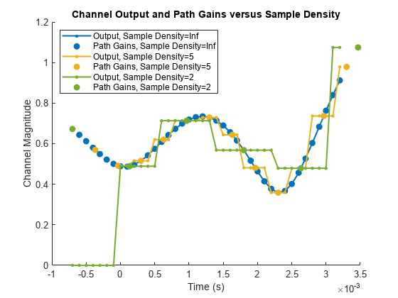
Plot channel output and path gain snapshots for various sample density values while using an lte3DChannel System object.

Configure a 3-D channel for SISO operation and delay profile CDL-B from TR 38.901 Section 7.7.1. Set the maximum Doppler shift to 300 Hz and the channel sampling rate to 10 kHz.

lte3d = lte3DChannel.makeCDL('CDL-B');
lte3d.MaximumDopplerShift = 300.0;
lte3d.SampleRate = 10e3;
lte3d.Seed = 19;

Configure transmit and receive antenna arrays.

lte3d.TransmitAntennaArray.Size = [1 1 1];
lte3d.ReceiveAntennaArray.Size = [1 1 1];

Create an input waveform with a length of 40 samples.

T = 40; 
in = ones(T,1); 

Plot the step response of the channel (displayed as lines) and the corresponding path gain snapshots (displayed circles) for various values of the SampleDensity property. The sample density property controls how often the channel snapshots are taken relative to the Doppler frequency.

  • When SampleDensity = Inf, a channel snapshot is taken for every input sample.

  • When SampleDensity = X, a channel snapshot is taken at a rate of Fcs = 2*X*MaximumDopplerShift.

The lte3DChannel object applies the channel snapshots to the input waveform by means of zero-order hold interpolation. The object takes an extra snapshot beyond the end of the input. Some of the final output samples use this extra value to minimize the interpolation error. The channel output contains a transient (and a delay) due to the filters that implement the path delays.

s = [Inf 5 2]; % sample densities
  
legends = {};
figure; hold on;
SR = lte3d.SampleRate;

for i = 1:length(s)
      
    % call channel with chosen sample density
    release(lte3d); lte3d.SampleDensity = s(i);
    [out,pathgains,sampletimes] = lte3d(in);
    chInfo = info(lte3d); tau = chInfo.ChannelFilterDelay;
      
    % plot channel output against time
    t = lte3d.InitialTime + ((0:(T-1)) - tau).' / SR;
    h = plot(t,abs(out),'o-'); h.MarkerSize = 2; h.LineWidth = 1.5;
    desc = ['Sample Density=' num2str(s(i))];
    legends = [legends ['Output, ' desc]];
    disp([desc ', Ncs=' num2str(length(sampletimes))]);
      
    % plot path gains against sample times
    h2 = plot(sampletimes - tau/SR,abs(sum(pathgains,2)),'o');
    h2.Color = h.Color; h2.MarkerFaceColor = h.Color;
    legends = [legends ['Path Gains, ' desc]];
      
end
Sample Density=Inf, Ncs=40
Sample Density=5, Ncs=13
Sample Density=2, Ncs=6
xlabel('Time (s)');
title('Channel Output and Path Gains versus Sample Density');
ylabel('Channel Magnitude');
legend(legends,'Location','NorthWest'); 

Figure contains an axes object. The axes object with title Channel Output and Path Gains versus Sample Density, xlabel Time (s), ylabel Channel Magnitude contains 6 objects of type line. One or more of the lines displays its values using only markers These objects represent Output, Sample Density=Inf, Path Gains, Sample Density=Inf, Output, Sample Density=5, Path Gains, Sample Density=5, Output, Sample Density=2, Path Gains, Sample Density=2.

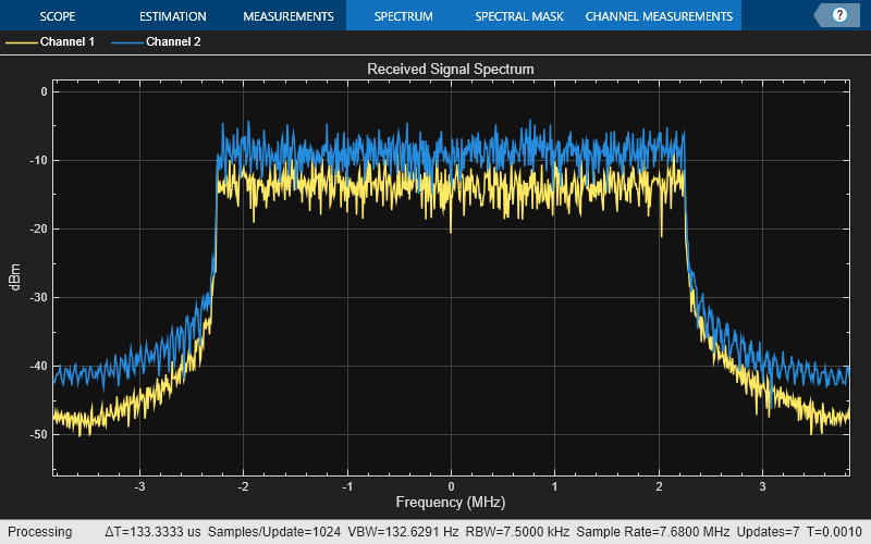
Display waveform spectrum of an LTE OFDM modulation waveform passed through a 40-by-2 channel using the lte3DChannel System object.

Create a resource grid for 40 antennas.

enb.NDLRB = 25;
enb.CyclicPrefix = 'Normal';
grid = lteDLResourceGrid(enb,40);
Fill the grid with QPSK symbols and perform LTE OFDM modulation.
grid(:) = lteSymbolModulate(randi([0 1],numel(grid)*2,1),'QPSK');
[txWaveform,txInfo] = lteOFDMModulate(enb,grid);

Create an lte3DChannel System object with specific properties.

lte3d = lte3DChannel('PathDelays',[0 500e-9], ...
    'AveragePathGains',[-13.4 3.0], ...
    'AnglesAoD',[-178.1 -4.2], ...
    'AnglesAoA',[51.3 -152.7], ...
    'AnglesZoD',[50.2 93.2], ...
    'AnglesZoA',[125.4 91.3], ...
    'NumStrongestClusters',1, ...
    'SampleRate',txInfo.SamplingRate);

Configure transmit and receive antenna arrays.

lte3d.TransmitAntennaArray.Size = [10 2 2];
lte3d.ReceiveAntennaArray.Size = [1 1 2];

The antenna array elements are mapped to the waveform channels (columns) using linear indexing of TransmitAntennaArray.Size or ReceiveAntennaArray.Size across the first dimension to the last. See the TransmitAntennaArray or ReceiveAntennaArray properties of the lte3DChannel System object for more details.

Pass the LTE OFDM modulation waveform through the 40-by-2 3-D channel.

rxWaveform = lte3d(txWaveform);

Plot the received waveform spectrum.

analyzer = spectrumAnalyzer(SampleRate=lte3d.SampleRate);
analyzer.Title = 'Received Signal Spectrum';
analyzer(rxWaveform);

References

[1] 3GPP TR 36.873. “Study on 3D channel model for LTE.” 3rd Generation Partnership Project; Technical Specification Group Radio Access Network; Evolved Universal Terrestrial Radio Access (E-UTRA). URL: https://www.3gpp.org.

[2] 3GPP TR 38.901. “Study on channel model for frequencies from 0.5 to 100 GHz.” 3rd Generation Partnership Project; Technical Specification Group Radio Access Network. URL: https://www.3gpp.org.

Version History

Introduced in R2018a