Analyze Urban V2V Connectivity Using Proximity and Ray Tracing
R2026bThis example shows how to analyze vehicle-to-vehicle (V2V) connectivity in an urban environment.
In this example, you:
Create an urban scenario using buildings derived from OpenStreetMap® data.
Add vehicles to roads derived from OpenStreetMap data.
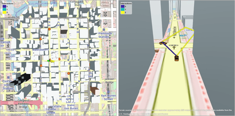
Visualize the scenario using side-by-side bird's-eye and ego-following views.
Analyze the proximity of the vehicles.
Analyze the V2V connectivity of the vehicles using geometric ray tracing.
Create Urban Scenario
Create a scenario for a region in Chicago.
Import Building, Road, and Basemap Data
Read the buildings and lines layers from an OpenStreetMap file [1] into geospatial tables. Extract common types of roads from the lines layer.
bldgslayer = readgeotable("chicago.osm",Layer="buildings");
lineslayer = readgeotable("chicago.osm",Layer="lines");

roadtypes = ["motorway","trunk","primary","secondary","tertiary","residential"];
roadrows = ismember(lineslayer.highway,roadtypes);
roads = lineslayer(roadrows,:);
Add a custom basemap from OpenStreetMap.
url = "a.tile.openstreetmap.org/${z}/${x}/${y}.png";
attr = string(char(169)) + "OpenStreetMap contributors";
addCustomBasemap("openstreetmap",url,Attribution=attr)
Preview Data
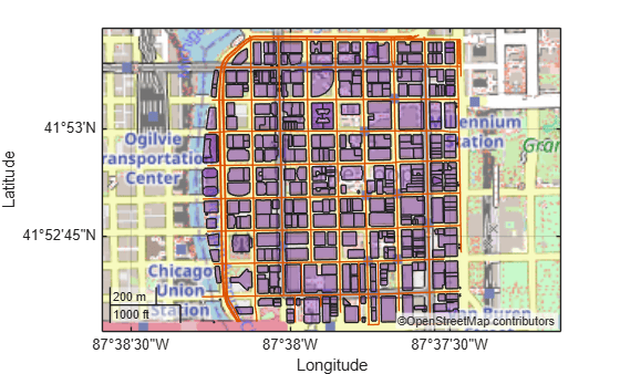
Preview the data by displaying the basemap, buildings, and roads on a 2D map.
figure
geobasemap openstreetmap
geoplot(bldgslayer,FaceColor=[0.45 0.1 0.7])
hold on
geoplot(roads)
Create Scenario
Add custom buildings from the imported data, then create the scenario. By default, the scenario uses terrain data from the GMTED2010 model.
addCustomBuildings("chicago",bldgslayer,NameExistsRule="preserve")
scnro = scenario(Buildings="chicago");
Add Vehicles to Roads
Generate traffic for the scenario using a simplified approach, with one vehicle per road segment and speeds that are proportional to the length of the road.
Select Roads for Traffic
Specify the corner coordinates of a rectangular area of interest (AOI) within the bounds of the OpenStreetMap file, then display the AOI on the 2D map.
aoi = aoiquad([41.8781 41.8846],[-87.6355 -87.6260]);
geoplot(aoi,FaceAlpha=0.4)
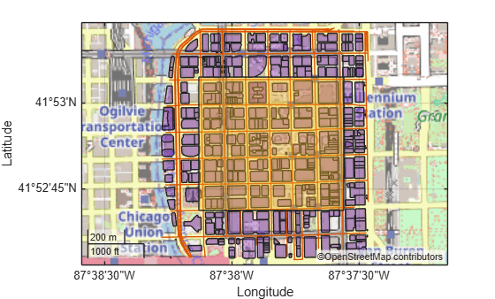
Clip the roads to the AOI, then replace the roads in the geospatial table with the clipped roads.
aoiroads = geoclip(roads.Shape,aoi);
roads.Shape = aoiroads;
Remove roads that are entirely outside the AOI.
isInAOI = roads.Shape.NumParts > 0;
roads(~isInAOI,:) = [];
Remove the short roads, so that the vehicles move for most of the simulation.
isShort = linelength(roads.Shape) < 200;
roads(isShort,:) = [];
Get Road Coordinates
Extract the geographic coordinates from the clipped roads. Calculate ground speeds that are proportional to the length of the road, up to 20 m/s (about 45 mph).
rdT = geotable2table(roads,["Latitude","Longitude"]);
rdlat = rdT.Latitude;
rdlon = rdT.Longitude;
rdlength = linelength(roads.Shape);

normlengths = rdlength/max(rdlength);
groundspeeds = max(1,round(normlengths*20));
Add Vehicles with Trajectories
Add a vehicle to each road segment. Generate the trajectory for each vehicle from the extracted road coordinates. Use the same simulation step size for each vehicle.
timestep = 0.2;
for k = 1:height(roads)
    waypts = pointtable(rdlat{k},rdlon{k});
    traj = groundTrajectory(waypts,GroundSpeed=groundspeeds(k));
    c = car(scnro,traj);
    c.Behavior.TimeStep = timestep;
end
Select an ego vehicle. Create separate variables for the ego vehicle and the other vehicles.
egoidx = 6;

egocar = scnro.Actors(egoidx);
othercars = scnro.Actors;
othercars(egoidx) = [];
Store the total number of vehicles and number of only non-ego vehicles for use in loops and variable initialization.
numCars = numel(scnro.Actors);
numOtherCars = numel(othercars);
Create Viewers
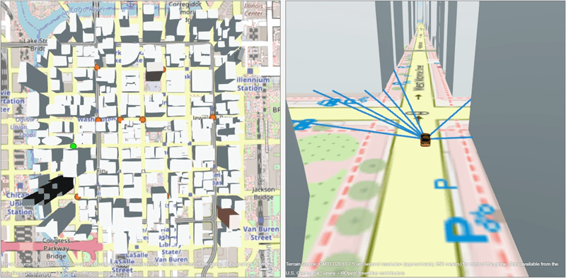
Visualize the scenario by creating a bird's-eye viewer and an ego-following viewer.
Create a figure with two side-by-side panels.
uif = uifigure(Position=[100 100 1200 600]);
ug = uigridlayout(uif,[1,2]);
p1 = uipanel(ug);
p2 = uipanel(ug);
Create Bird's-Eye Viewer
Add a viewer to the left panel. Create the bird's-eye view by moving the camera to look straight down from above.
vbird = viewer(scnro,Parent=p1,Basemap="openstreetmap", ...
    Name="Bird's-Eye Viewer");

campt = pointtable(41.881,-87.631,1500,HeightReference="ellipsoid");
campos(vbird,campt)
campitch(vbird,-90)
Distinguish the ego vehicle from the other vehicles by changing the color of its marker.
egovis = getvisual(vbird,egocar);
egovis.MarkerFaceColor = "green";
Store the visuals for the non-ego vehicles and the default marker color in variables. Use these variables to change the appearances of the vehicles during simulation.
othervisuals = scenario.graphics.ActorVisual.empty;
for k = 1:numel(othercars)
    othervisuals(k) = getvisual(vbird,othercars(k));
end

defaultmarker = othervisuals(1).MarkerFaceColor;
Simplify the visualization by hiding the trajectory of each vehicle.
for k = 1:numCars
    act = scnro.Actors(k);
    actvis = getvisual(vbird,act.Behavior);
    actvis.Visible = false;
end
Create Ego Viewer
Add a viewer to the right panel. Create the ego-following view by moving the camera behind the vehicle.
vego = viewer(scnro,Parent=p2,Name="Ego Viewer",Basemap="openstreetmap");
follow(vego,egocar,Offset=[-40 0 20])
Display a line between the ego vehicle and each other vehicle.
egopt = position(egocar);
otherpts = position(othercars);

linevisuals = scenario.graphics.LineVisual.empty;
for k = 1:numOtherCars
    otherpt = otherpts(k,:);
    linevisuals(k) = plotline(vego,[egopt; otherpt],LineWidth=3);
end
Store the default line color in a variable. Use this variable to change the appearances of the lines during simulation.
defaultcolor = linevisuals(1).Color;
Simplify the visualization by hiding the trajectory of each vehicle.
for k = 1:numCars
    actvis = getvisual(vego,scnro.Actors(k).Behavior);
    actvis.Visible = false;
end
Analyze Proximity
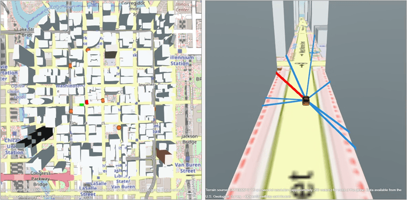
Analyze how close other vehicles get to the ego vehicle over time. Use minimum separation distance to identify which vehicles are candidates for detection or communication.
Run Proximity Simulation
Prepare to run the proximity simulation:
Get the body frame of the ego vehicle, which is useful for calculating relative distances.
Initialize variables that, at each time step, store the simulation time and minimum distance.
egoframe = bodyframe(egocar);
simtimes = [];
mindists = [];
Run the proximity simulation in a loop. At each time step:
Get the position of each vehicle, in geographic coordinates. Get the pose of each non-ego vehicle with respect to the ego vehicle.
Calculate the distance between the centroid of the ego vehicle and the centroid of each other vehicle.
Update the endpoints of the line visuals.
Update the visual for each vehicle based on proximity, such that the closest vehicle has a red marker and a thick red line. The farther vehicles have thinner lines.
Record the simulation time and the minimum distance between the ego vehicle and the other vehicles.
while advance(scnro)
    % Get vehicle positions and poses
    egopt = position(egocar);
    otherpts = position(othercars);
    otherptscart = pose(othercars,ReferenceFrame=egoframe);

    dists = zeros(numOtherCars,1);
    for k = 1:numOtherCars
        % Calculate distance from each vehicle to ego vehicle
        dists(k) = norm(otherptscart(k).Position);
        otherpt = otherpts(k,:);

        % Update endpoints of line visuals
        linevisuals(k).Data = [egopt; otherpt];

        % Update line widths
        rr = rescale(dists(k),InputMin=0,InputMax=500);
        linevisuals(k).LineWidth = 3 + round((1-rr)*3);
    end

    [mindist,nearest] = min(dists);
    for k = 1:numOtherCars
        % Highlight closest vehicle using red marker and line
        if k == nearest
            linevisuals(k).Color = "red";
            othervisuals(k).MarkerFaceColor = "red";
        % Reset colors of farther vehicles
        else
            linevisuals(k).Color = defaultcolor;
            othervisuals(k).MarkerFaceColor = defaultmarker;
        end
    end

    % Record simulation time and minimum distance
    simtimes = [simtimes; scnro.SimulationTime]; %#ok<AGROW>
    mindists = [mindists; mindist]; %#ok<AGROW>
end
Plot Minimum Separation Distance
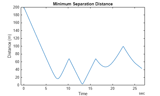
Plot the minimum separation distance over time. The shortest separation occurs about 13 seconds into the simulation, when two vehicles pass through the same intersection.
figure
plot(simtimes,mindists)
xlabel("Time")
ylabel("Distance (m)")
title("Minimum Separation Distance")
Analyze V2V Connectivity
The proximity analysis identifies nearby vehicles, but does not account for building occlusion. Determine which candidates are connectable by adding a ray trace analysis that models signal paths through the scenario.
Reset Simulation
Reset the simulation by hiding the proximity lines, resetting the marker colors, and restarting the scenario.
for k = 1:numOtherCars
    linevisuals(k).Visible = false;
    othervisuals(k).MarkerFaceColor = defaultmarker;
end

restart(scnro)
Set Up Ray Trace Analysis
Create a ray trace analysis that finds geometric paths from the front bumper of the ego vehicle to the roofs of the other vehicles. Set up the analysis to find direct paths, one-bounce reflections, and two-bounce reflections. This combination approximates realistic V2V radio link paths in an urban canyon.
rt = rayTraceAnalysis(egocar,othercars,MaxNumReflections=2, ...
    SourceReferencePoint="frontbumper",DestinationReferencePoint="roof");
Run Ray Trace Simulation
Prepare to run the ray trace simulation by initializing a variable that, at each time step, stores the connectivity.
connectivity = false(0,numOtherCars);
Run the simulation again. At each time step:
Find ray paths from the ego vehicle to the other vehicles.
Determine if the vehicles are connectable. A vehicle is connectable if at least one valid path exists.
Record the connectivity.
while advance(scnro)
    % Find ray paths
    pathsets = findpaths(rt);

    % Determine if vehicles are connectable
    connectable = false(1,numel(pathsets));
    for k = 1:numel(pathsets)
        connectable(k) = ~isempty(pathsets(k).Paths);
    end

    % Record connectivity
    connectivity = [connectivity; connectable]; %#ok<AGROW>
end
Plot V2V Link Connectivity
Plot the connectivity of each vehicle over time. For each non-ego vehicle, display a horizontal line at the time steps where a viable communication path exists.
figure
hold on
for k = 1:numOtherCars
    y = repmat(k,size(simtimes));
    y(~connectivity(:,k)) = NaN;
    plot(simtimes,y,LineWidth=3)
end
hold off
Customize the plot by adding tick labels, a title, and a grid.
yticks(1:numOtherCars)
yticklabels("Car " + setdiff(1:numCars,egoidx))

xlabel("Time")

title("V2V Link Connectivity")

grid on
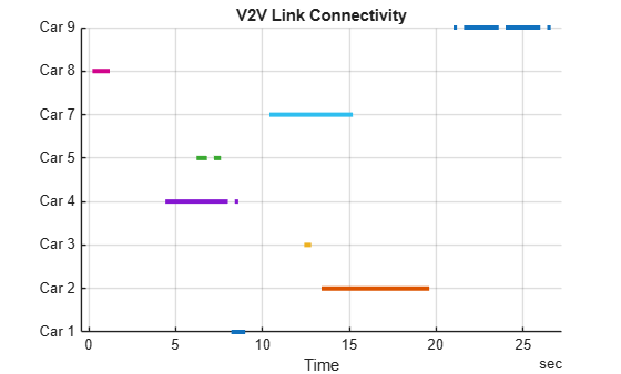
Gaps in the line indicate time steps where buildings occlude all paths between the ego vehicle and that vehicle. Most vehicles are only intermittently connectable.
References
[1] You can download OpenStreetMap files from https://www.openstreetmap.org, which provides access to crowd-sourced map data all over the world. The data is licensed under the Open Data Commons Open Database License (ODbL), https://opendatacommons.org/licenses/odbl/.
See Also
scenario | viewer | car | rayTraceAnalysis | findpaths

